
33 minutes
Written: 2020-01-15 05:28 +0000
ISLR :: Multiple Linear Regression
Chapter II - Statistical Learning
All the questions are as per the ISL seventh printing of the First edition 1.
Question 2.8 - Pages 54-55
This exercise relates to the College data set, which can be found in
the file College.csv. It contains a number of variables for \(777\)
different universities and colleges in the US. The variables are
Private: Public/private indicatorApps: Number of applications receivedAccept: Number of applicants acceptedEnroll: Number of new students enrolledTop10perc: New students from top 10 % of high school classTop25perc: New students from top 25 % of high school classF.Undergrad: Number of full-time undergraduatesP.Undergrad: Number of part-time undergraduatesOutstate: Out-of-state tuitionRoom.Board: Room and board costsBooks: Estimated book costsPersonal: Estimated personal spendingPhD: Percent of faculty with Ph.D.’sTerminal: Percent of faculty with terminal degreeS.F.Ratio: Student/faculty ratioperc.alumni: Percent of alumni who donateExpend: Instructional expenditure per studentGrad.Rate: Graduation rate
Before reading the data into R, it can be viewed in Excel or a text editor.
(a) Use the read.csv() function to read the data into R . Call the
loaded data college. Make sure that you have the directory set to the
correct location for the data.
(b) Look at the data using the fix() function. You should notice
that the first column is just the name of each university. We don’t
really want R to treat this as data. However, it may be handy to have
these names for later. Try the following commands:
1rownames(college)=college[,1]
2fix(college)
You should see that there is now a row.names column with the name of each university recorded. This means that R has given each row a name corresponding to the appropriate university. R will not try to perform calculations on the row names. However, we still need to eliminate the first column in the data where the names are stored. Try:
1college=college[,-1]
2fix(college)
(c)
- Use the
summary()function to produce a numerical summary of the variables in the data set. - Use the
pairs()function to produce a scatterplot matrix of the first ten columns or variables of the data. Recall that you can reference the first ten columns of a matrixAusingA[,1:10]. - Use the
plot()function to produce side-by-side boxplots of Outstate versus Private . - Create a new qualitative variable, called Elite , by binning the
Top10percvariable. We are going to divide universities into two groups based on whether or not the proportion of students coming from the top \(10%\) of their high school classes exceeds \(50%\).
1Elite = rep("No", nrow(college))
2Elite [college$Top10perc >50]="Yes"
3Elite = as.factor (Elite)
4college = data.frame (college, Elite)
Use the summary() function to see how many elite univer- sities there
are. Now use the plot() function to produce side-by-side boxplots of
Outstate versus Elite .
- Use the hist() function to produce some histograms with differing
numbers of bins for a few of the quantitative vari- ables. You may
fnd the command
par(mfrow=c(2,2))useful: it will divide the print window into four regions so that four plots can be made simultaneously. Modifying the arguments to this function will divide the screen in other ways. - Continue exploring the data, and provide a brief summary of what you discover.
Answer
Instead of reading in data, for ISLR in particular we can load the ISLR library which is on CRAN and contains the data-sets required for the book.
1install.packages("ISLR")
Thus, we can now read it in as library("ISLR")
The remaining sections are meant to be executed, and are marked as such,
with r in {}.
(c)
We will load the dataset once for the whole document.
1library("ISLR")
- Usage of the
summary()function
1summary(ISLR::College)
 1##  Private        Apps           Accept          Enroll       Top10perc
 2##  No :212   Min.   :   81   Min.   :   72   Min.   :  35   Min.   : 1.00
 3##  Yes:565   1st Qu.:  776   1st Qu.:  604   1st Qu.: 242   1st Qu.:15.00
 4##            Median : 1558   Median : 1110   Median : 434   Median :23.00
 5##            Mean   : 3002   Mean   : 2019   Mean   : 780   Mean   :27.56
 6##            3rd Qu.: 3624   3rd Qu.: 2424   3rd Qu.: 902   3rd Qu.:35.00
 7##            Max.   :48094   Max.   :26330   Max.   :6392   Max.   :96.00
 8##    Top25perc      F.Undergrad     P.Undergrad         Outstate
 9##  Min.   :  9.0   Min.   :  139   Min.   :    1.0   Min.   : 2340
10##  1st Qu.: 41.0   1st Qu.:  992   1st Qu.:   95.0   1st Qu.: 7320
11##  Median : 54.0   Median : 1707   Median :  353.0   Median : 9990
12##  Mean   : 55.8   Mean   : 3700   Mean   :  855.3   Mean   :10441
13##  3rd Qu.: 69.0   3rd Qu.: 4005   3rd Qu.:  967.0   3rd Qu.:12925
14##  Max.   :100.0   Max.   :31643   Max.   :21836.0   Max.   :21700
15##    Room.Board       Books           Personal         PhD
16##  Min.   :1780   Min.   :  96.0   Min.   : 250   Min.   :  8.00
17##  1st Qu.:3597   1st Qu.: 470.0   1st Qu.: 850   1st Qu.: 62.00
18##  Median :4200   Median : 500.0   Median :1200   Median : 75.00
19##  Mean   :4358   Mean   : 549.4   Mean   :1341   Mean   : 72.66
20##  3rd Qu.:5050   3rd Qu.: 600.0   3rd Qu.:1700   3rd Qu.: 85.00
21##  Max.   :8124   Max.   :2340.0   Max.   :6800   Max.   :103.00
22##     Terminal       S.F.Ratio      perc.alumni        Expend
23##  Min.   : 24.0   Min.   : 2.50   Min.   : 0.00   Min.   : 3186
24##  1st Qu.: 71.0   1st Qu.:11.50   1st Qu.:13.00   1st Qu.: 6751
25##  Median : 82.0   Median :13.60   Median :21.00   Median : 8377
26##  Mean   : 79.7   Mean   :14.09   Mean   :22.74   Mean   : 9660
27##  3rd Qu.: 92.0   3rd Qu.:16.50   3rd Qu.:31.00   3rd Qu.:10830
28##  Max.   :100.0   Max.   :39.80   Max.   :64.00   Max.   :56233
29##    Grad.Rate
30##  Min.   : 10.00
31##  1st Qu.: 53.00
32##  Median : 65.00
33##  Mean   : 65.46
34##  3rd Qu.: 78.00
35##  Max.   :118.00
- Usage of
pairs()
1tenColl <- ISLR::College[,1:10] # For getting the first ten columns
2pairs(tenColl) # Scatterplot
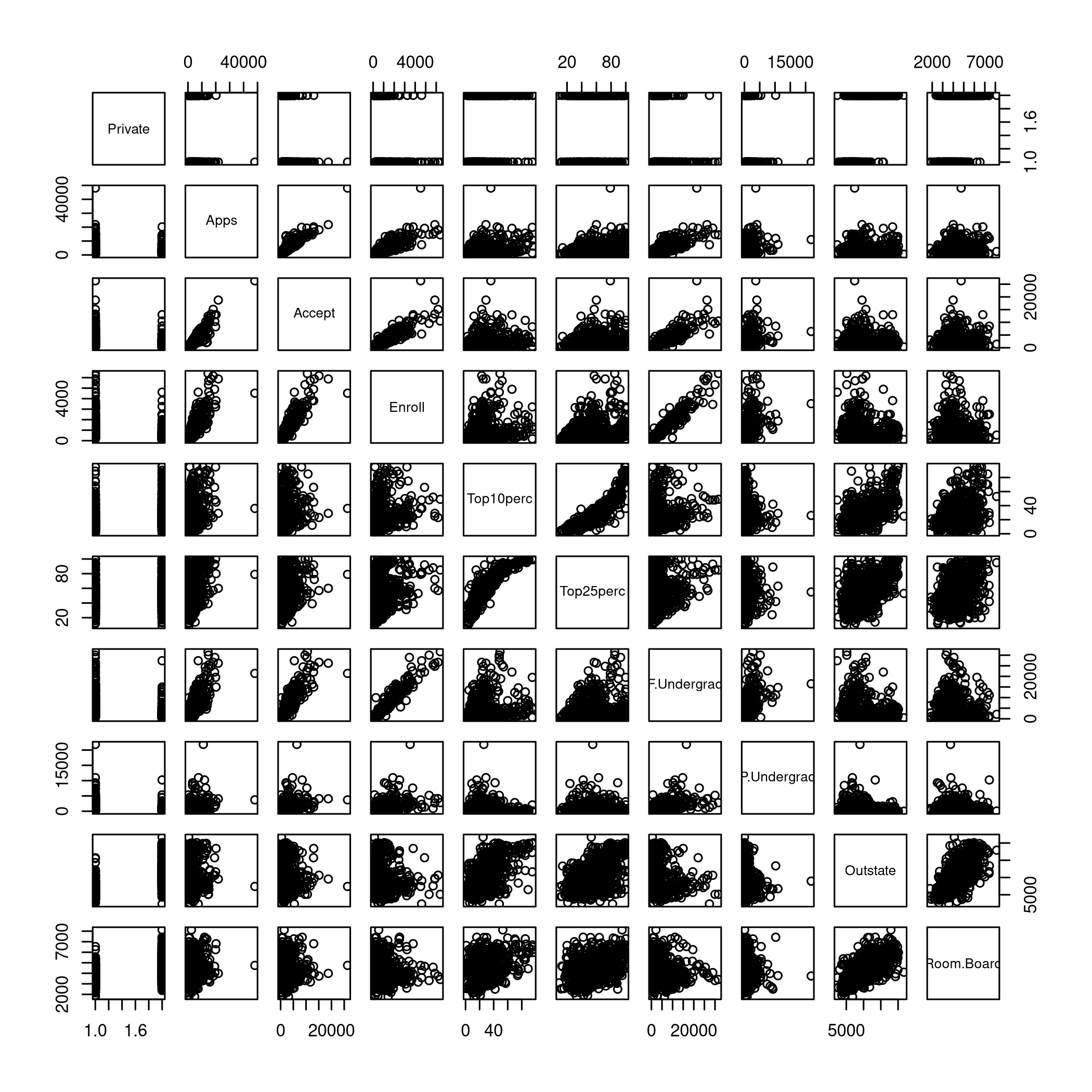
Figure 1: Pairs
- Boxplot creation with
plot()
1plot(ISLR::College$Private,ISLR::College$Outstate,xlab="Private",ylab="Outstate")
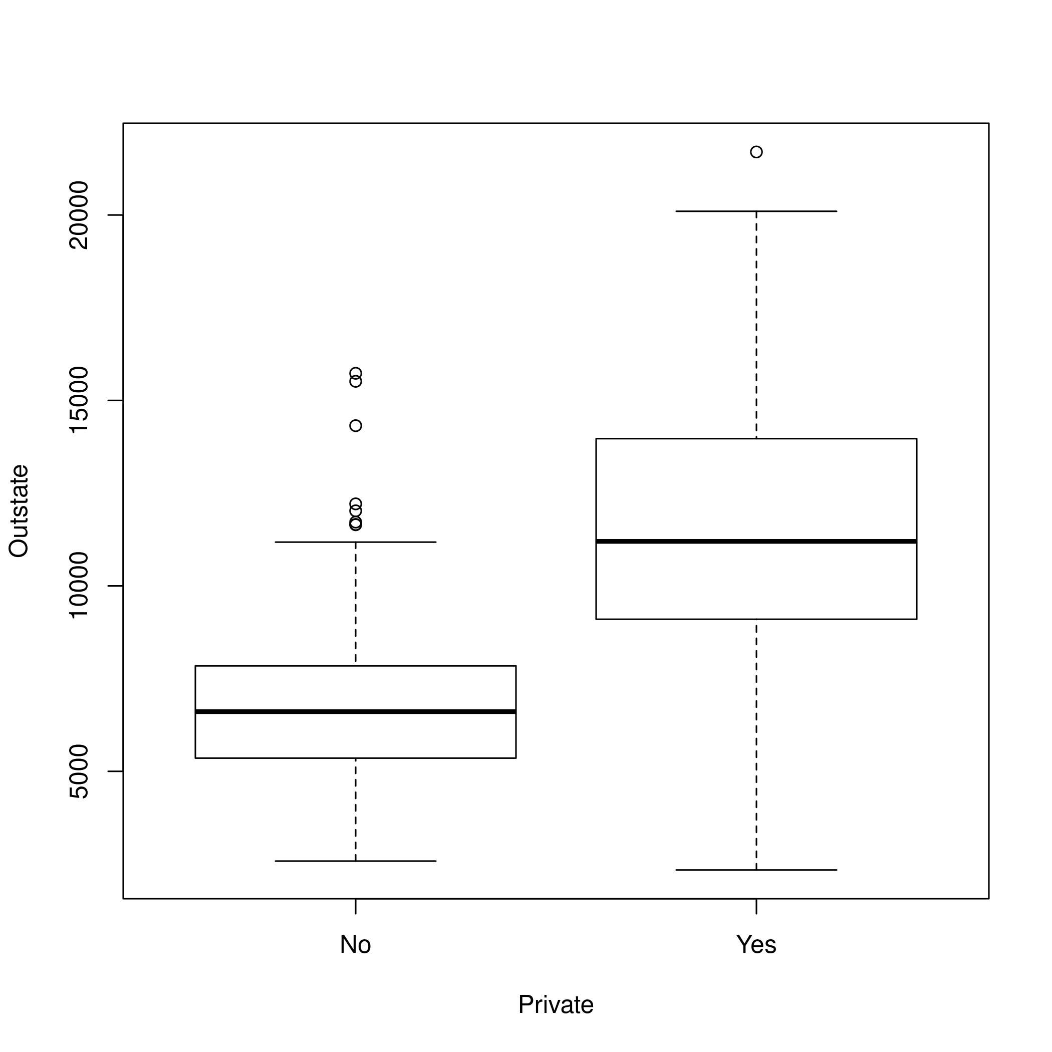
Figure 2: Boxplots
- Binning and plotting
1college=ISLR::College
2Elite=rep("No",nrow(college))
3Elite[college$Top10perc>50]="Yes"
4Elite=as.factor(Elite)
5college<-data.frame(college,Elite)
6summary(college$Elite)
1##  No Yes
2## 699  78
1plot(college$Outstate,college$Elite,xlab="Outstate",ylab="Elite")
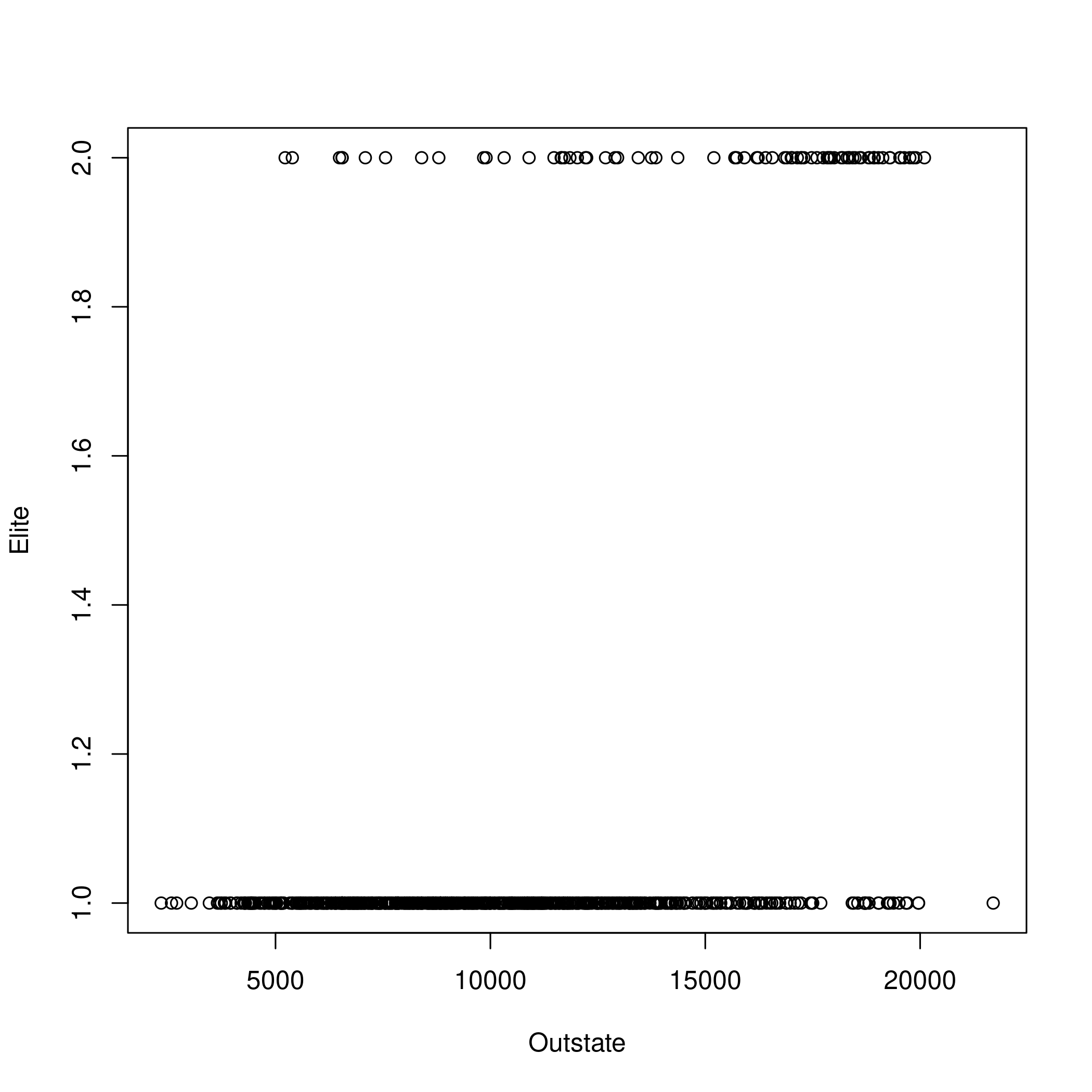
Figure 3: Plotting Outstate and Elite
- Histograms with
hist()
1par(mfrow=c(2,2))
2hist(college$Enroll)
3hist(college$perc.alumni, col=2)
4hist(college$Personal, col=3, breaks=10)
5hist(college$PhD, breaks=10)
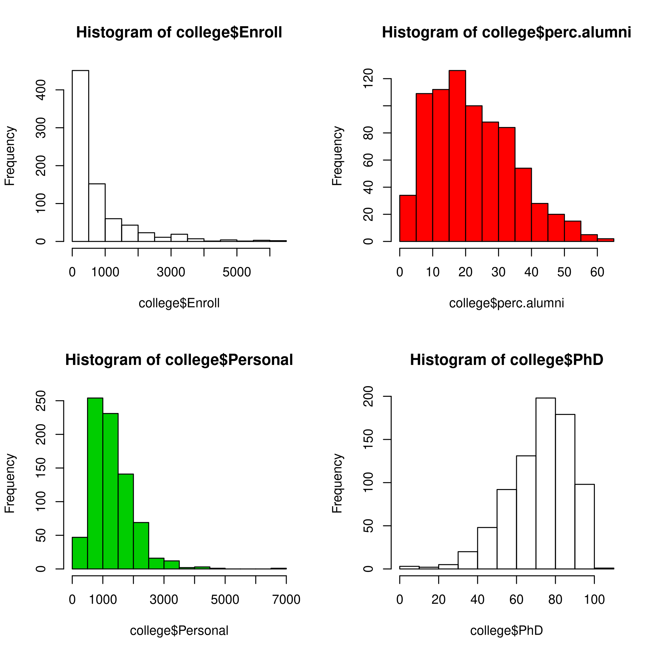
Figure 4: Histogram
1hist(college$Top10perc, col="blue")
2hist(college$Outstate, col=23)
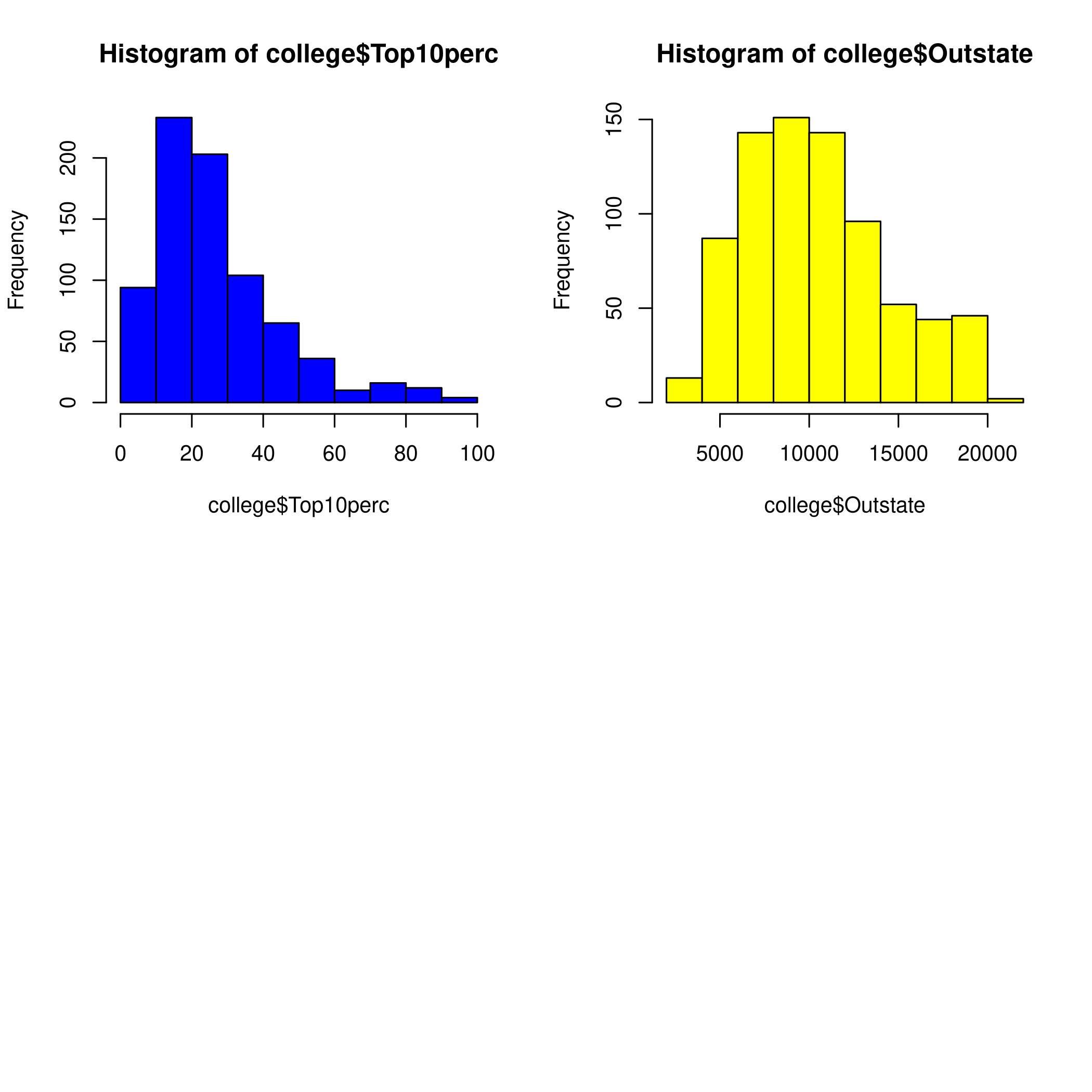
Figure 5: Colored Histogram
- Explorations (graphical)
\(0\) implies the faculty have PhDs. It is clear that people donate more when faculty do not have terminal degrees.
1plot(college$Terminal-college$PhD, college$perc.alumni)
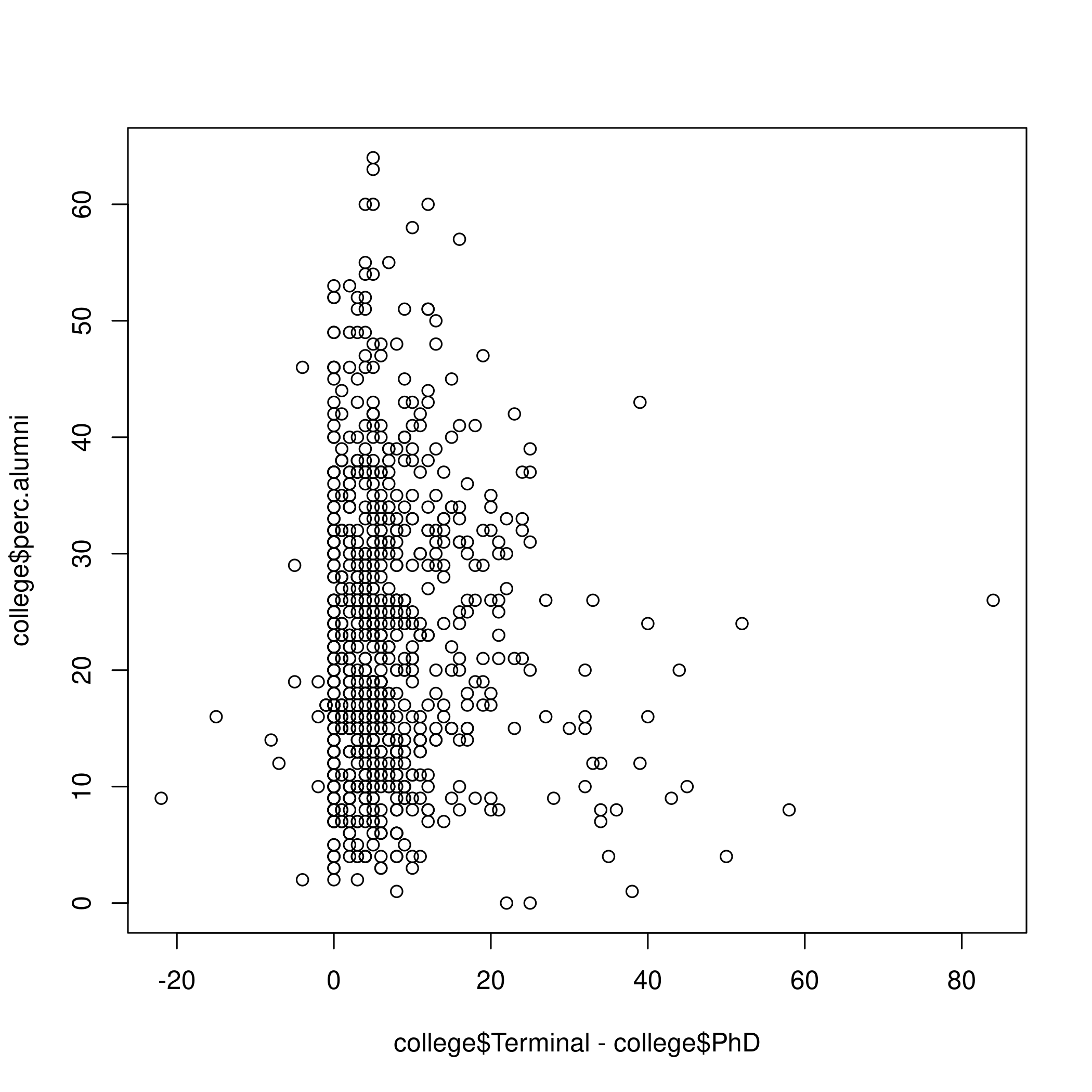
Figure 6: Terminal degrees and alumni
High tuition correlates to high graduation rate.
1plot(college$Expend, college$Grad.Rate)
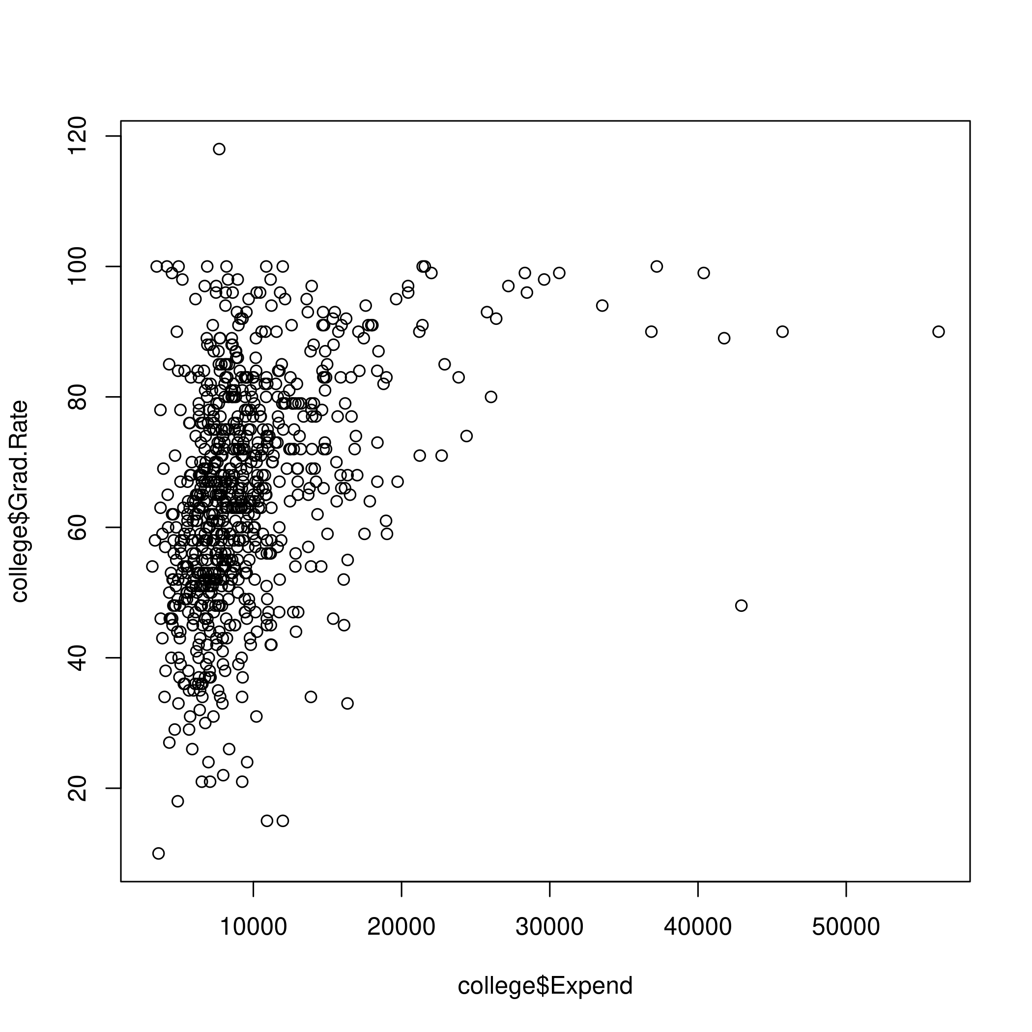
Figure 7: Tuiton and graduation
Low acceptance implies a low student to faculty ratio.
1plot(college$Accept / college$Apps, college$S.F.Ratio)
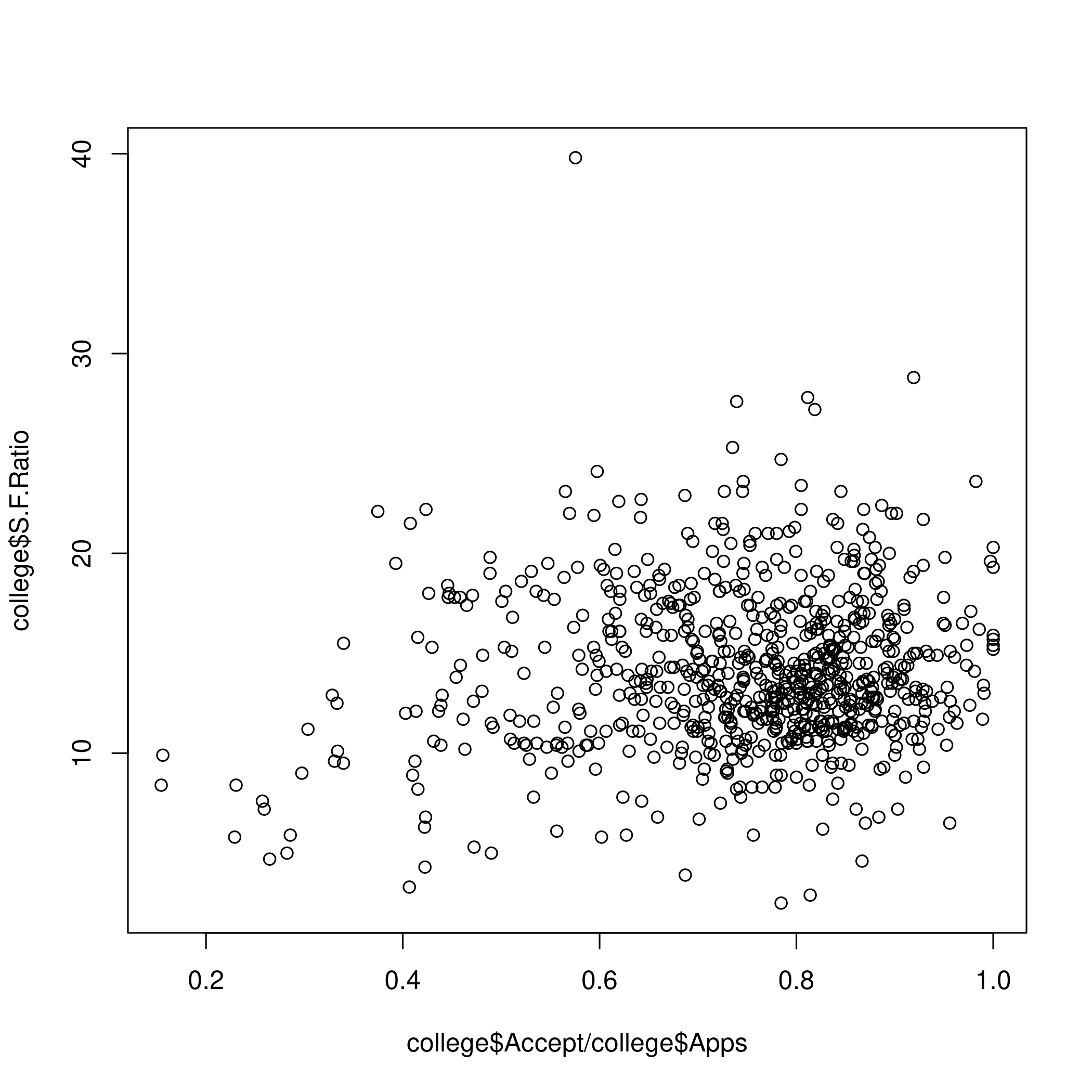
Figure 8: Acceptance and Student/Faculty ratio
Question 2.9 - Page 56
This exercise involves the Auto data set studied in the lab. Make sure
that the missing values have been removed from the data.
(a) Which of the predictors are quantitative, and which are qualitative?
(b) What is the range of each quantitative predictor? You can answer
this using the range() function.
(c) What is the mean and standard deviation of each quantitative predictor?
(d) Now remove the 10th through 85th observations. What is the range, mean, and standard deviation of each predictor in the subset of the data that remains?
(e) Using the full data set, investigate the predictors graphically, using scatterplots or other tools of your choice. Create some plots highlighting the relationships among the predictors. Comment on your findings.
(f) Suppose that we wish to predict gas mileage (mpg) on the basis
of the other variables. Do your plots suggest that any of the other
variables might be useful in predicting mpg? Justify your answer.
Answer
Once again, since the dataset is loaded from the library, we will simply start manipulating it.
1# Clean data
2autoDat<-na.omit(ISLR::Auto) # renamed for convenience
(a) To determine weather the variables a qualitative or quantitative we can either inspect the variables by eye, or query the dataset.
1summary(autoDat) # Observe the output for variance
 1##       mpg          cylinders      displacement     horsepower        weight
 2##  Min.   : 9.00   Min.   :3.000   Min.   : 68.0   Min.   : 46.0   Min.   :1613
 3##  1st Qu.:17.00   1st Qu.:4.000   1st Qu.:105.0   1st Qu.: 75.0   1st Qu.:2225
 4##  Median :22.75   Median :4.000   Median :151.0   Median : 93.5   Median :2804
 5##  Mean   :23.45   Mean   :5.472   Mean   :194.4   Mean   :104.5   Mean   :2978
 6##  3rd Qu.:29.00   3rd Qu.:8.000   3rd Qu.:275.8   3rd Qu.:126.0   3rd Qu.:3615
 7##  Max.   :46.60   Max.   :8.000   Max.   :455.0   Max.   :230.0   Max.   :5140
 8##
 9##   acceleration        year           origin                      name
10##  Min.   : 8.00   Min.   :70.00   Min.   :1.000   amc matador       :  5
11##  1st Qu.:13.78   1st Qu.:73.00   1st Qu.:1.000   ford pinto        :  5
12##  Median :15.50   Median :76.00   Median :1.000   toyota corolla    :  5
13##  Mean   :15.54   Mean   :75.98   Mean   :1.577   amc gremlin       :  4
14##  3rd Qu.:17.02   3rd Qu.:79.00   3rd Qu.:2.000   amc hornet        :  4
15##  Max.   :24.80   Max.   :82.00   Max.   :3.000   chevrolet chevette:  4
16##                                                  (Other)           :365
1str(autoDat) # Directly find find out
 1## 'data.frame':    392 obs. of  9 variables:
 2##  $ mpg         : num  18 15 18 16 17 15 14 14 14 15 ...
 3##  $ cylinders   : num  8 8 8 8 8 8 8 8 8 8 ...
 4##  $ displacement: num  307 350 318 304 302 429 454 440 455 390 ...
 5##  $ horsepower  : num  130 165 150 150 140 198 220 215 225 190 ...
 6##  $ weight      : num  3504 3693 3436 3433 3449 ...
 7##  $ acceleration: num  12 11.5 11 12 10.5 10 9 8.5 10 8.5 ...
 8##  $ year        : num  70 70 70 70 70 70 70 70 70 70 ...
 9##  $ origin      : num  1 1 1 1 1 1 1 1 1 1 ...
10##  $ name        : Factor w/ 304 levels "amc ambassador brougham",..: 49 36 231 14 161 141 54 223 241 2 ...
From the above view, we can see that there is only one listed as a
qualitative variable or factor, and that is name. However, we can also
do this in a cleaner manner or at-least in a different manner with a
function.
1findFactors <- sapply(autoDat,is.factor)
2findFactors
1##          mpg    cylinders displacement   horsepower       weight acceleration
2##        FALSE        FALSE        FALSE        FALSE        FALSE        FALSE
3##         year       origin         name
4##        FALSE        FALSE         TRUE
Though only name is listed as a qualitative variable, we note that origin seems to be almost qualitative as well.
1length(unique(autoDat$origin))
1## [1] 3
1unique(autoDat$origin)
1## [1] 1 3 2
Infact we can check that nothing else has this property by repeated
application of sapply, though a pipe would be more satisfying
1getUniq<-sapply(autoDat, unique)
2getLengths<-sapply(getUniq,length)
3getLengths
1##          mpg    cylinders displacement   horsepower       weight acceleration
2##          127            5           81           93          346           95
3##         year       origin         name
4##           13            3          301
This is really nicer with pipes
1library(dplyr)
1##
2## Attaching package: 'dplyr'
1## The following objects are masked from 'package:stats':
2##
3##     filter, lag
1## The following objects are masked from 'package:base':
2##
3##     intersect, setdiff, setequal, union
1autoDat %>% sapply(unique) %>% sapply(length)
1##          mpg    cylinders displacement   horsepower       weight acceleration
2##          127            5           81           93          346           95
3##         year       origin         name
4##           13            3          301
At any rate, we know now that origin and name are probably qualitative, and the rest are quantitative.
(b) Using range()
A nice feature of the dataset we have is that the suspected qualitative variables are at the end of the dataset. So we can simply select the first \(7\) rows and go nuts on them.
1autoDat[,1:7] %>% sapply(range) # or sapply(autoDat[,1:7],range)
1##       mpg cylinders displacement horsepower weight acceleration year
2## [1,]  9.0         3           68         46   1613          8.0   70
3## [2,] 46.6         8          455        230   5140         24.8   82
Once again, more elegant with pipes and subset()
1autoDat %>% subset(select=-c(name,origin)) %>% sapply(range)
1##       mpg cylinders displacement horsepower weight acceleration year
2## [1,]  9.0         3           68         46   1613          8.0   70
3## [2,] 46.6         8          455        230   5140         24.8   82
1# Even simpler with dplyr
2autoDat %>% select(-name,-origin) %>% sapply(range)
1##       mpg cylinders displacement horsepower weight acceleration year
2## [1,]  9.0         3           68         46   1613          8.0   70
3## [2,] 46.6         8          455        230   5140         24.8   82
(c) Mean and standard deviation
1noFactors <- autoDat %>% select(-name,-origin)
2noFactors %>% sapply(mean)
1##          mpg    cylinders displacement   horsepower       weight acceleration
2##    23.445918     5.471939   194.411990   104.469388  2977.584184    15.541327
3##         year
4##    75.979592
1noFactors %>% sapply(sd)
1##          mpg    cylinders displacement   horsepower       weight acceleration
2##     7.805007     1.705783   104.644004    38.491160   849.402560     2.758864
3##         year
4##     3.683737
(d) Removing observations 10-85 and testing.
1noFactors[-(10:85),] %>% sapply(mean)
1##          mpg    cylinders displacement   horsepower       weight acceleration
2##    24.404430     5.373418   187.240506   100.721519  2935.971519    15.726899
3##         year
4##    77.145570
1noFactors[-(10:85),] %>% sapply(sd)
1##          mpg    cylinders displacement   horsepower       weight acceleration
2##     7.867283     1.654179    99.678367    35.708853   811.300208     2.693721
3##         year
4##     3.106217
(e) Plots for determining relationships
1par(mfrow=c(2,2))
2plot(autoDat$weight, autoDat$horsepower)
3plot(autoDat$weight, autoDat$acceleration)
4plot(autoDat$displacement, autoDat$acceleration)
5plot(autoDat$cylinders, autoDat$acceleration)
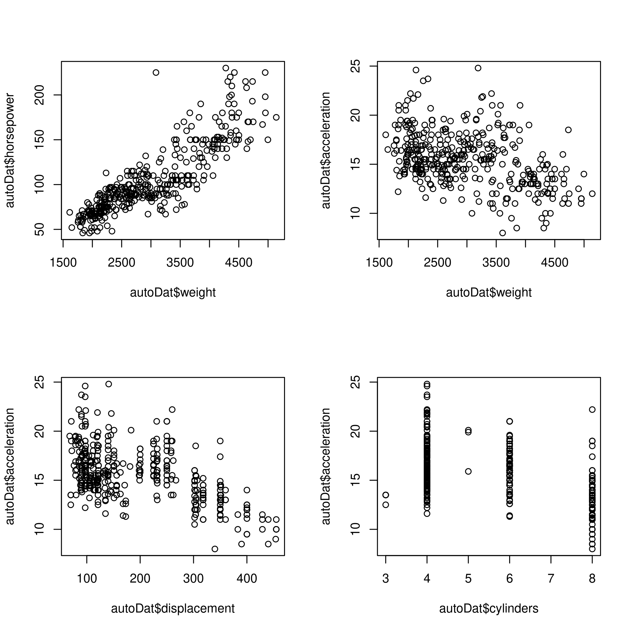
Figure 9: Relationship determination
- Evidently horsepower is directly proportional to weight but acceleration is inversely proportional to weight
- Acceleration is also inversely proportional to displacement
- Cylinders are a poor measure, not surprising since there are only \(5\) values
(f) Choosing predictors for gas mileage mpg
Let us recall certain key elements of the quantitative aspects of the dataset.
1summary(noFactors) # To understand the spread
 1##       mpg          cylinders      displacement     horsepower        weight
 2##  Min.   : 9.00   Min.   :3.000   Min.   : 68.0   Min.   : 46.0   Min.   :1613
 3##  1st Qu.:17.00   1st Qu.:4.000   1st Qu.:105.0   1st Qu.: 75.0   1st Qu.:2225
 4##  Median :22.75   Median :4.000   Median :151.0   Median : 93.5   Median :2804
 5##  Mean   :23.45   Mean   :5.472   Mean   :194.4   Mean   :104.5   Mean   :2978
 6##  3rd Qu.:29.00   3rd Qu.:8.000   3rd Qu.:275.8   3rd Qu.:126.0   3rd Qu.:3615
 7##  Max.   :46.60   Max.   :8.000   Max.   :455.0   Max.   :230.0   Max.   :5140
 8##   acceleration        year
 9##  Min.   : 8.00   Min.   :70.00
10##  1st Qu.:13.78   1st Qu.:73.00
11##  Median :15.50   Median :76.00
12##  Mean   :15.54   Mean   :75.98
13##  3rd Qu.:17.02   3rd Qu.:79.00
14##  Max.   :24.80   Max.   :82.00
1getLengths # To get the number of unique values
1##          mpg    cylinders displacement   horsepower       weight acceleration
2##          127            5           81           93          346           95
3##         year       origin         name
4##           13            3          301
From this we can assert easily that the number of cylinders is not of much interest for predictions of the mileage.
1par(mfrow=c(3,2))
2plot(noFactors$mpg,noFactors$horsepower)
3plot(noFactors$mpg,noFactors$weight)
4plot(noFactors$mpg,noFactors$displacement)
5plot(noFactors$mpg,noFactors$acceleration)
6plot(noFactors$mpg,noFactors$year)
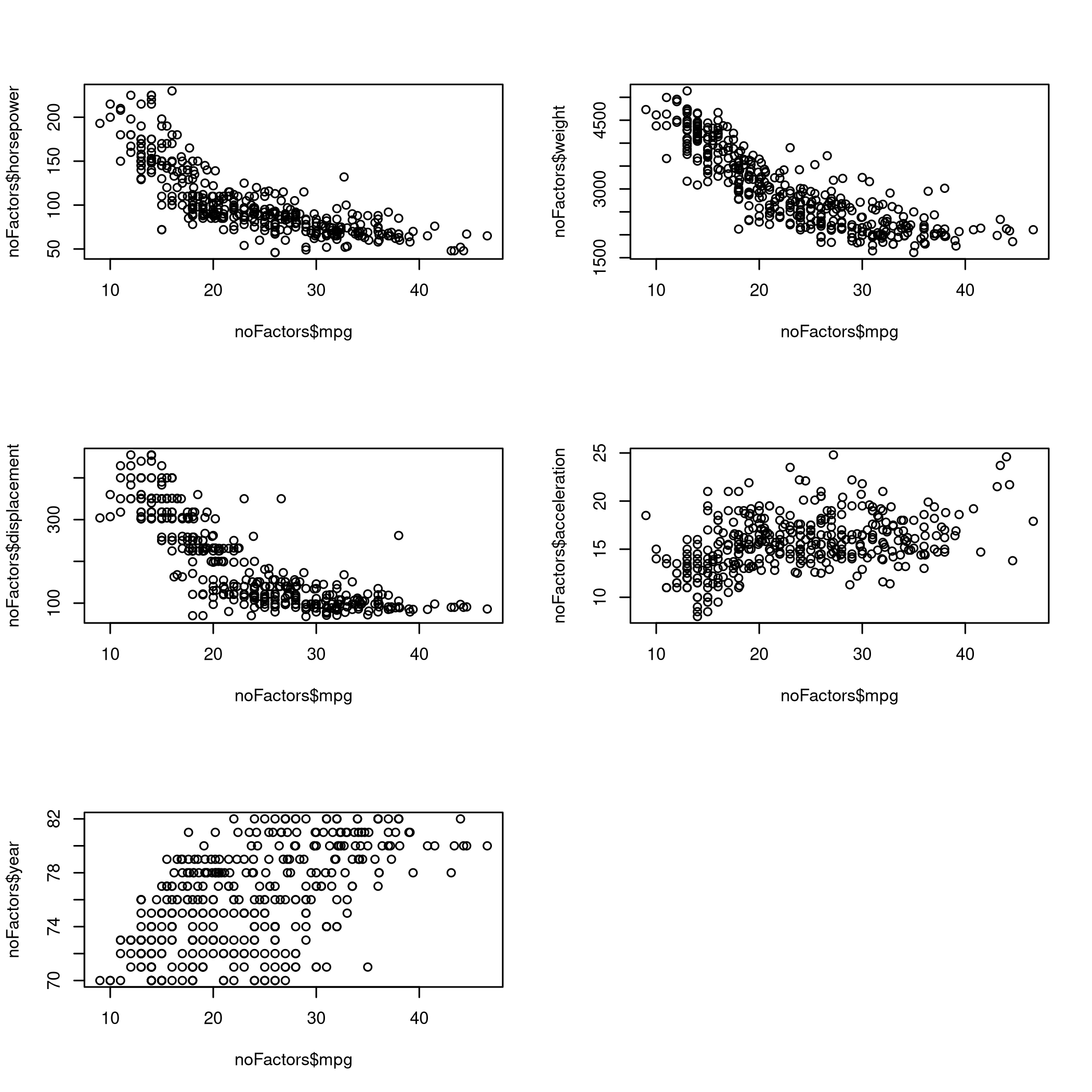
Figure 10: Predictions
- So now we know that the mileage increases when horsepower is low, weight is low, displacement is low and acceleration is high
Where low represents an inverse response and high represents a direct response.
- It is also clear that the mileage increases every year
Chapter III - Linear Regression
Question 3.9 - Page 122
This question involves the use of multiple linear regression on the Auto data set.
(a) Produce a scatterplot matrix which includes all of the variables in the data set.
(b) Compute the matrix of correlations between the variables using the
function cor() . You will need to exclude the name variable, cor()
which is qualitative.
(c) Use the lm() function to perform a multiple linear regression
with mpg as the response and all other variables except name as the
predictors. Use the summary() function to print the results. Comment
on the output. For instance:
- Is there a relationship between the predictors and the response?
- Which predictors appear to have a statistically significant relationship to the response?
- What does the coefficient for the year variable suggest?
(d) Use the plot() function to produce diagnostic plots of the
linear regression fit. Comment on any problems you see with the fit. Do
the residual plots suggest any unusually large outliers? Does the
leverage plot identify any observations with unusually high leverage?
(e) Use the * and : symbols to fit linear regression models with
interaction effects. Do any interactions appear to be statistically
significant?
(f) Try a few different transformations of the variables, such as \(\log{X}\), \(\sqrt{X}\), \(X^2\).Comment on your findings.
Answer
Once again, we will use the dataset from the library.
1cleanAuto <- na.omit(autoDat)
2summary(cleanAuto) # Already created above, so no need to do na.omit again
 1##       mpg          cylinders      displacement     horsepower        weight
 2##  Min.   : 9.00   Min.   :3.000   Min.   : 68.0   Min.   : 46.0   Min.   :1613
 3##  1st Qu.:17.00   1st Qu.:4.000   1st Qu.:105.0   1st Qu.: 75.0   1st Qu.:2225
 4##  Median :22.75   Median :4.000   Median :151.0   Median : 93.5   Median :2804
 5##  Mean   :23.45   Mean   :5.472   Mean   :194.4   Mean   :104.5   Mean   :2978
 6##  3rd Qu.:29.00   3rd Qu.:8.000   3rd Qu.:275.8   3rd Qu.:126.0   3rd Qu.:3615
 7##  Max.   :46.60   Max.   :8.000   Max.   :455.0   Max.   :230.0   Max.   :5140
 8##
 9##   acceleration        year           origin                      name
10##  Min.   : 8.00   Min.   :70.00   Min.   :1.000   amc matador       :  5
11##  1st Qu.:13.78   1st Qu.:73.00   1st Qu.:1.000   ford pinto        :  5
12##  Median :15.50   Median :76.00   Median :1.000   toyota corolla    :  5
13##  Mean   :15.54   Mean   :75.98   Mean   :1.577   amc gremlin       :  4
14##  3rd Qu.:17.02   3rd Qu.:79.00   3rd Qu.:2.000   amc hornet        :  4
15##  Max.   :24.80   Max.   :82.00   Max.   :3.000   chevrolet chevette:  4
16##                                                  (Other)           :365
(a) Scatterplot
1pairs(cleanAuto)
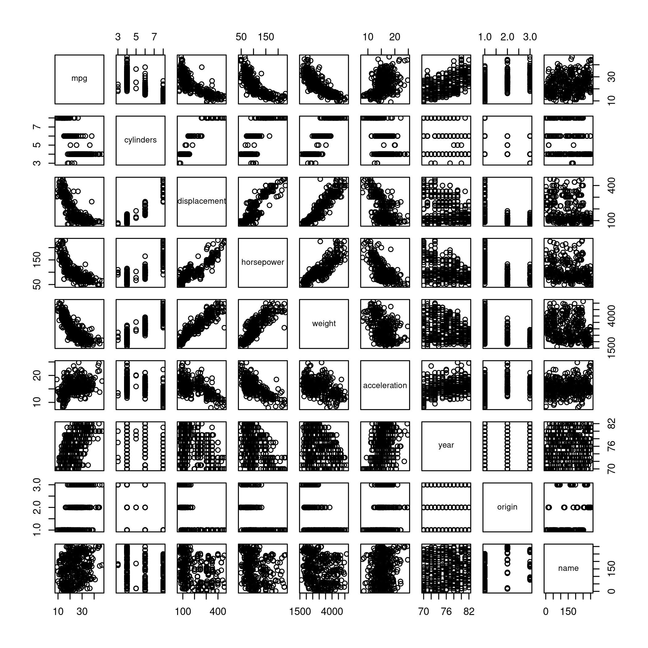
Figure 11: Scatterplot
(b) Correlation matrix. For this we exclude the qualitative variables
either by using select or by using the existing noFactors dataset
1# A full set
2ISLR::Auto %>% na.omit %>% select(-name,-origin) %>% cor
 1##                     mpg  cylinders displacement horsepower     weight
 2## mpg           1.0000000 -0.7776175   -0.8051269 -0.7784268 -0.8322442
 3## cylinders    -0.7776175  1.0000000    0.9508233  0.8429834  0.8975273
 4## displacement -0.8051269  0.9508233    1.0000000  0.8972570  0.9329944
 5## horsepower   -0.7784268  0.8429834    0.8972570  1.0000000  0.8645377
 6## weight       -0.8322442  0.8975273    0.9329944  0.8645377  1.0000000
 7## acceleration  0.4233285 -0.5046834   -0.5438005 -0.6891955 -0.4168392
 8## year          0.5805410 -0.3456474   -0.3698552 -0.4163615 -0.3091199
 9##              acceleration       year
10## mpg             0.4233285  0.5805410
11## cylinders      -0.5046834 -0.3456474
12## displacement   -0.5438005 -0.3698552
13## horsepower     -0.6891955 -0.4163615
14## weight         -0.4168392 -0.3091199
15## acceleration    1.0000000  0.2903161
16## year            0.2903161  1.0000000
(c) Multiple Linear Regression
1# Fit against every variable
2lm.fit=lm(mpg~.,data=noFactors)
3summary(lm.fit)
 1##
 2## Call:
 3## lm(formula = mpg ~ ., data = noFactors)
 4##
 5## Residuals:
 6##     Min      1Q  Median      3Q     Max
 7## -8.6927 -2.3864 -0.0801  2.0291 14.3607
 8##
 9## Coefficients:
10##                Estimate Std. Error t value Pr(>|t|)
11## (Intercept)  -1.454e+01  4.764e+00  -3.051  0.00244 **
12## cylinders    -3.299e-01  3.321e-01  -0.993  0.32122
13## displacement  7.678e-03  7.358e-03   1.044  0.29733
14## horsepower   -3.914e-04  1.384e-02  -0.028  0.97745
15## weight       -6.795e-03  6.700e-04 -10.141  < 2e-16 ***
16## acceleration  8.527e-02  1.020e-01   0.836  0.40383
17## year          7.534e-01  5.262e-02  14.318  < 2e-16 ***
18## ---
19## Signif. codes:  0 '***' 0.001 '**' 0.01 '*' 0.05 '.' 0.1 ' ' 1
20##
21## Residual standard error: 3.435 on 385 degrees of freedom
22## Multiple R-squared:  0.8093, Adjusted R-squared:  0.8063
23## F-statistic: 272.2 on 6 and 385 DF,  p-value: < 2.2e-16
1# Fit against one variable
2noFactors %>% lm(mpg~horsepower,data=.) %>% summary
 1##
 2## Call:
 3## lm(formula = mpg ~ horsepower, data = .)
 4##
 5## Residuals:
 6##      Min       1Q   Median       3Q      Max
 7## -13.5710  -3.2592  -0.3435   2.7630  16.9240
 8##
 9## Coefficients:
10##              Estimate Std. Error t value Pr(>|t|)
11## (Intercept) 39.935861   0.717499   55.66   <2e-16 ***
12## horsepower  -0.157845   0.006446  -24.49   <2e-16 ***
13## ---
14## Signif. codes:  0 '***' 0.001 '**' 0.01 '*' 0.05 '.' 0.1 ' ' 1
15##
16## Residual standard error: 4.906 on 390 degrees of freedom
17## Multiple R-squared:  0.6059, Adjusted R-squared:  0.6049
18## F-statistic: 599.7 on 1 and 390 DF,  p-value: < 2.2e-16
1noFactors %>% lm(mpg~year,data=.) %>% summary
 1##
 2## Call:
 3## lm(formula = mpg ~ year, data = .)
 4##
 5## Residuals:
 6##      Min       1Q   Median       3Q      Max
 7## -12.0212  -5.4411  -0.4412   4.9739  18.2088
 8##
 9## Coefficients:
10##              Estimate Std. Error t value Pr(>|t|)
11## (Intercept) -70.01167    6.64516  -10.54   <2e-16 ***
12## year          1.23004    0.08736   14.08   <2e-16 ***
13## ---
14## Signif. codes:  0 '***' 0.001 '**' 0.01 '*' 0.05 '.' 0.1 ' ' 1
15##
16## Residual standard error: 6.363 on 390 degrees of freedom
17## Multiple R-squared:  0.337,  Adjusted R-squared:  0.3353
18## F-statistic: 198.3 on 1 and 390 DF,  p-value: < 2.2e-16
1noFactors %>% lm(mpg~acceleration,data=.) %>% summary
 1##
 2## Call:
 3## lm(formula = mpg ~ acceleration, data = .)
 4##
 5## Residuals:
 6##     Min      1Q  Median      3Q     Max
 7## -17.989  -5.616  -1.199   4.801  23.239
 8##
 9## Coefficients:
10##              Estimate Std. Error t value Pr(>|t|)
11## (Intercept)    4.8332     2.0485   2.359   0.0188 *
12## acceleration   1.1976     0.1298   9.228   <2e-16 ***
13## ---
14## Signif. codes:  0 '***' 0.001 '**' 0.01 '*' 0.05 '.' 0.1 ' ' 1
15##
16## Residual standard error: 7.08 on 390 degrees of freedom
17## Multiple R-squared:  0.1792, Adjusted R-squared:  0.1771
18## F-statistic: 85.15 on 1 and 390 DF,  p-value: < 2.2e-16
1noFactors %>% lm(mpg~weight,data=.) %>% summary
 1##
 2## Call:
 3## lm(formula = mpg ~ weight, data = .)
 4##
 5## Residuals:
 6##      Min       1Q   Median       3Q      Max
 7## -11.9736  -2.7556  -0.3358   2.1379  16.5194
 8##
 9## Coefficients:
10##              Estimate Std. Error t value Pr(>|t|)
11## (Intercept) 46.216524   0.798673   57.87   <2e-16 ***
12## weight      -0.007647   0.000258  -29.64   <2e-16 ***
13## ---
14## Signif. codes:  0 '***' 0.001 '**' 0.01 '*' 0.05 '.' 0.1 ' ' 1
15##
16## Residual standard error: 4.333 on 390 degrees of freedom
17## Multiple R-squared:  0.6926, Adjusted R-squared:  0.6918
18## F-statistic: 878.8 on 1 and 390 DF,  p-value: < 2.2e-16
1noFactors %>% lm(mpg~displacement,data=.) %>% summary
 1##
 2## Call:
 3## lm(formula = mpg ~ displacement, data = .)
 4##
 5## Residuals:
 6##      Min       1Q   Median       3Q      Max
 7## -12.9170  -3.0243  -0.5021   2.3512  18.6128
 8##
 9## Coefficients:
10##              Estimate Std. Error t value Pr(>|t|)
11## (Intercept)  35.12064    0.49443   71.03   <2e-16 ***
12## displacement -0.06005    0.00224  -26.81   <2e-16 ***
13## ---
14## Signif. codes:  0 '***' 0.001 '**' 0.01 '*' 0.05 '.' 0.1 ' ' 1
15##
16## Residual standard error: 4.635 on 390 degrees of freedom
17## Multiple R-squared:  0.6482, Adjusted R-squared:  0.6473
18## F-statistic: 718.7 on 1 and 390 DF,  p-value: < 2.2e-16
Clearly there is a relationship between the predictors and variables, mostly as described previously, with the following broad trends:
- Inversely proportional to Horsepower, Weight, and Displacement
The predictors which have a relationship to the response are (based on R squared values): \[ all > weight > displacement > horsepower > year > acceleration \] However, things lower than horsepower are not statistically significant.
The visual analysis of the
yearvariable suggests that the mileage grows every year. However, it is clear from the summary, that there is no statistical significance of year when used to fit a single parameter linear model. We note that when we compare this to the multiple linear regression analysis, we see that the year factor accounts for \(0.7508\) of the total, that is, the cars become more efficient every year
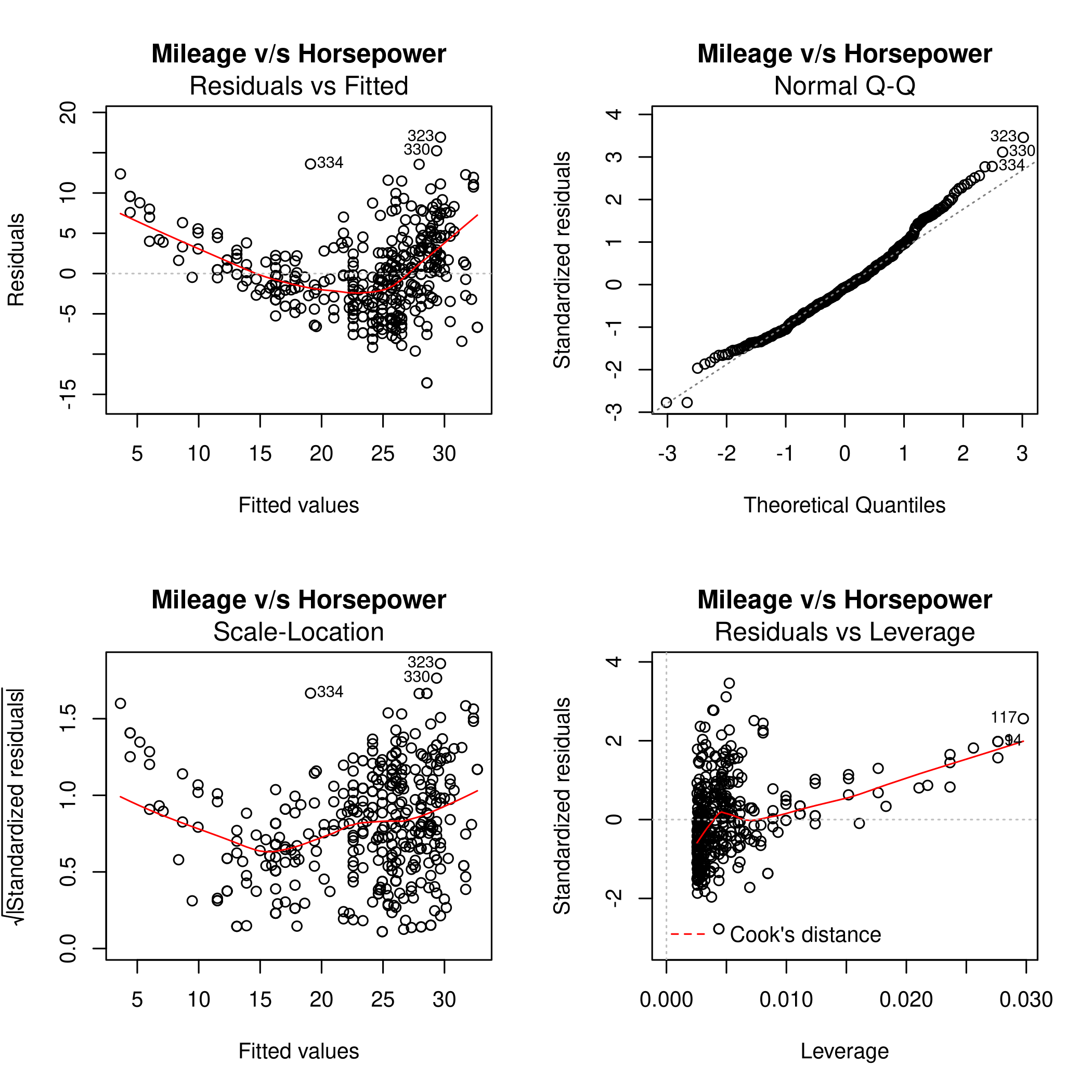
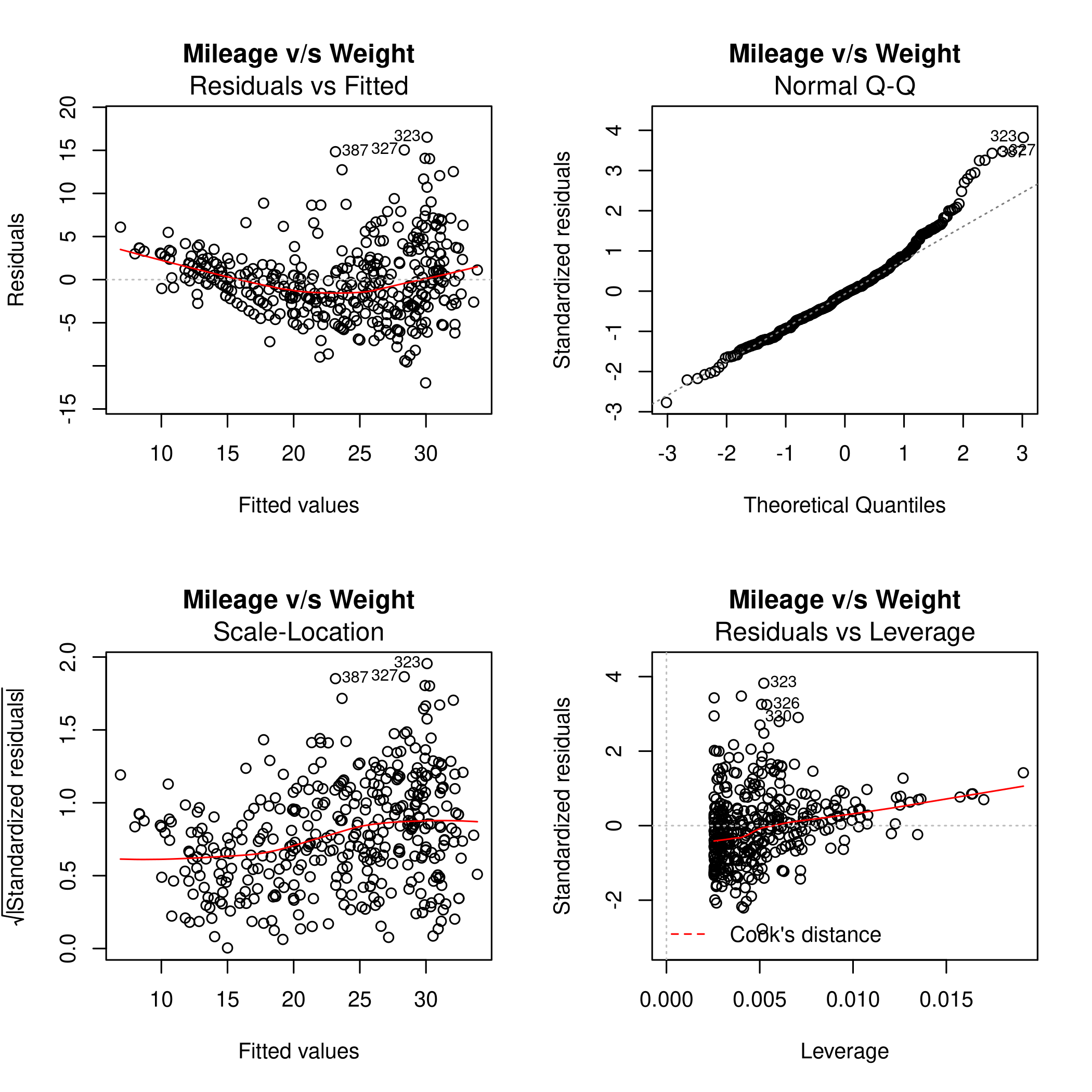
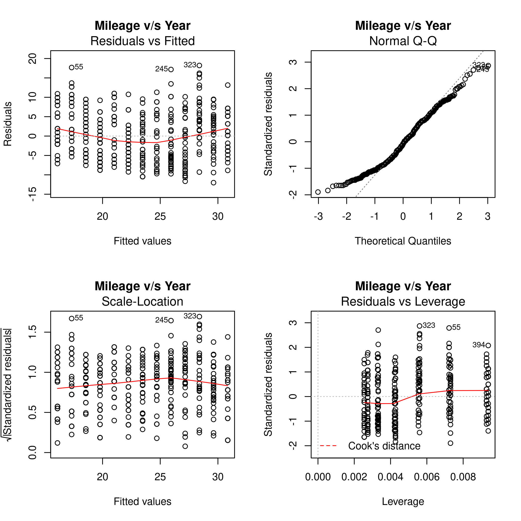
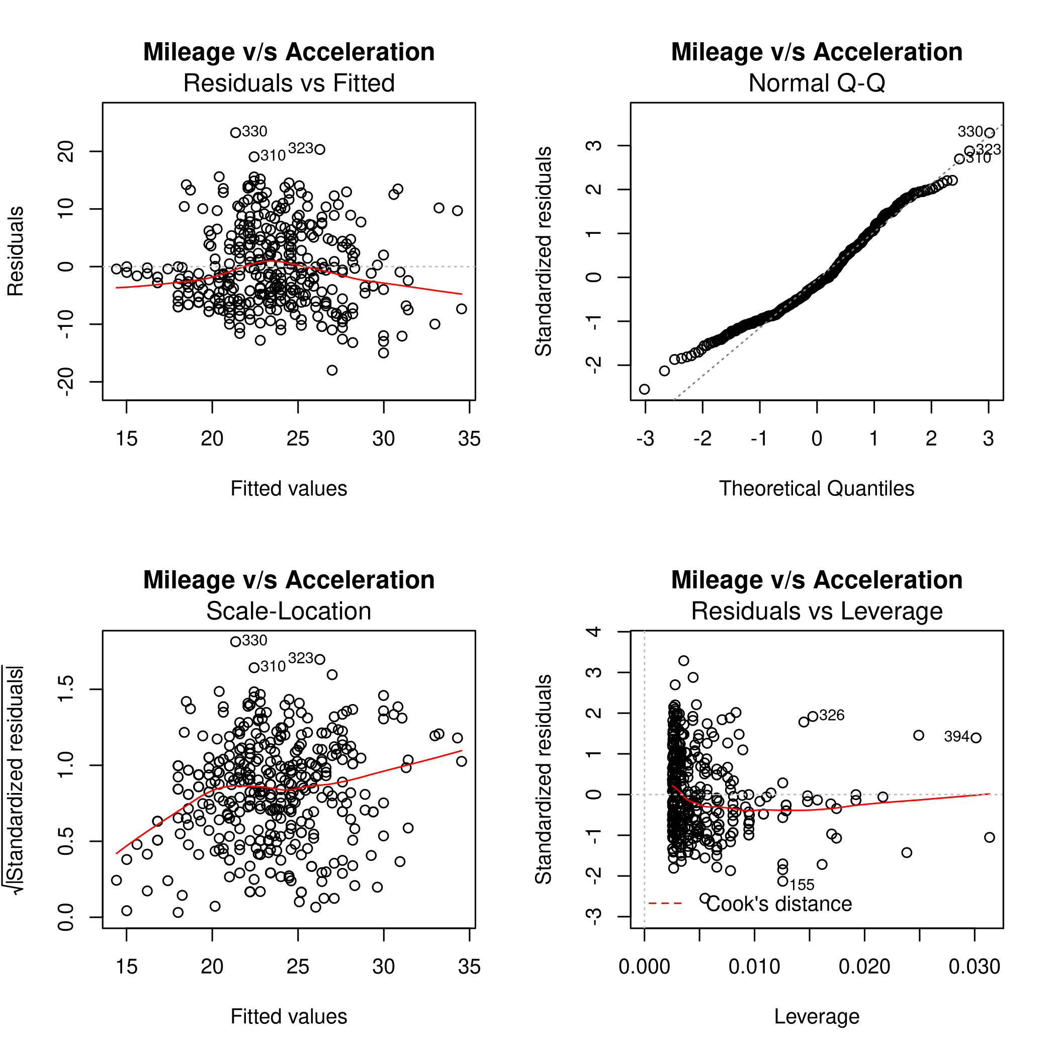
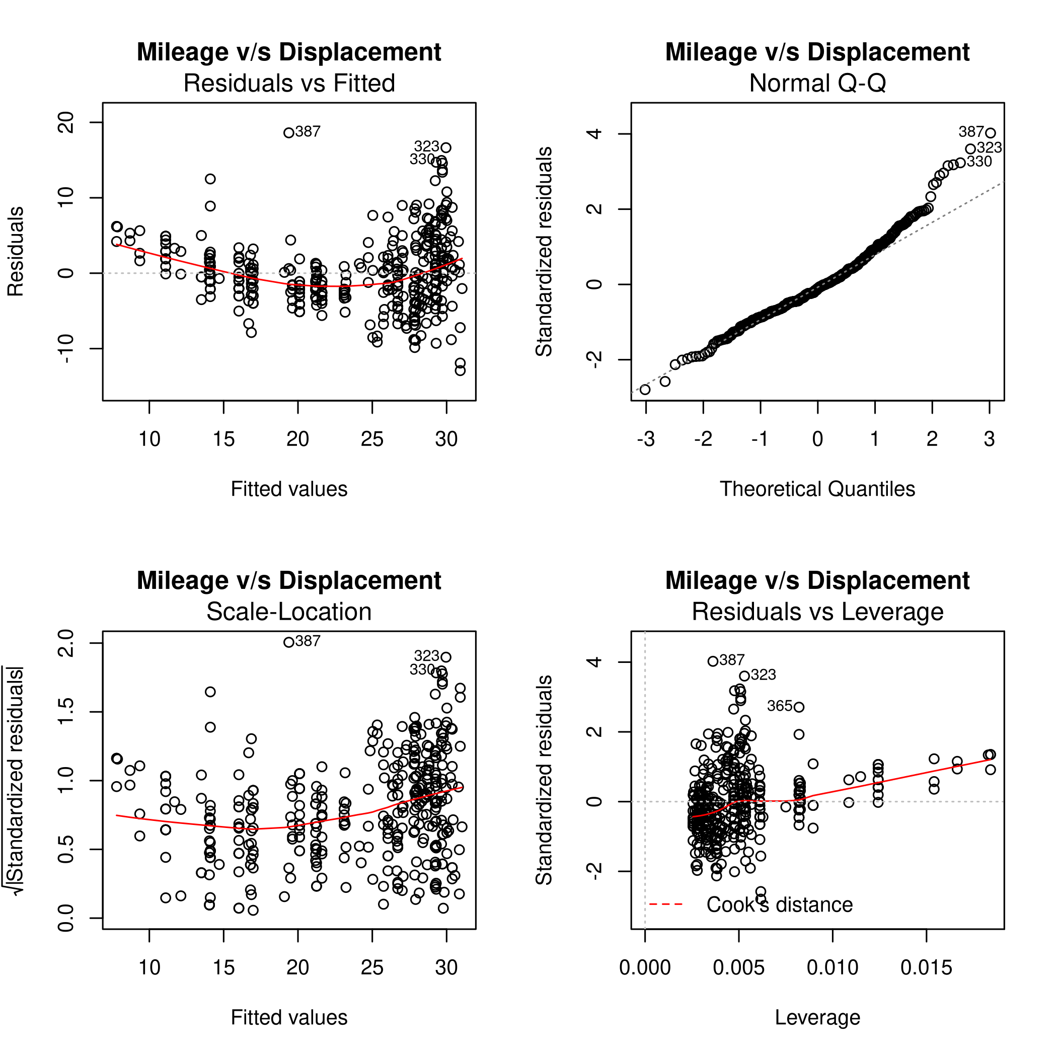
(d) Lets plot these
1par(mfrow=c(2,2))
2noFactors %>% lm(mpg~horsepower,data=.) %>% plot(main="Mileage v/s Horsepower")
1noFactors %>% lm(mpg~weight,data=.) %>% plot(main="Mileage v/s Weight")
1noFactors %>% lm(mpg~year,data=.) %>% plot(main="Mileage v/s Year")
1noFactors %>% lm(mpg~acceleration,data=.) %>% plot(main="Mileage v/s Acceleration")
1noFactors %>% lm(mpg~displacement,data=.) %>% plot(main="Mileage v/s Displacement")
1noFactors %>% lm(mpg~.,data=.) %>% plot(main="Mileage Multiple Regression")
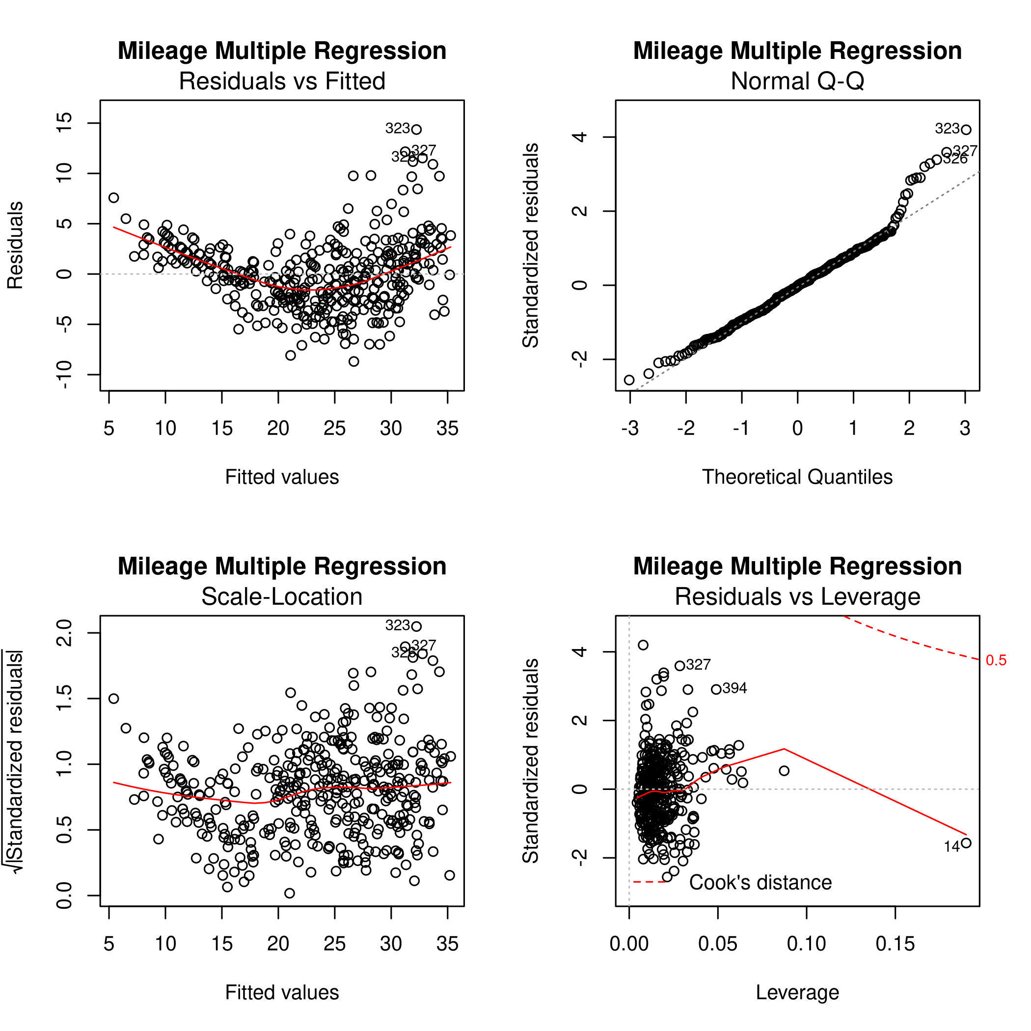
Form this we can see that the fit is not very accurate as there is a clear curve to the residuals. The 14th point has high leverage, though it is of a small magnitude. Thus it is not expected to have affected the plot too much.
We know that an observation with a studentized residual greater than \(3\) in absolute value are possible outliers. Hence we must plot this.
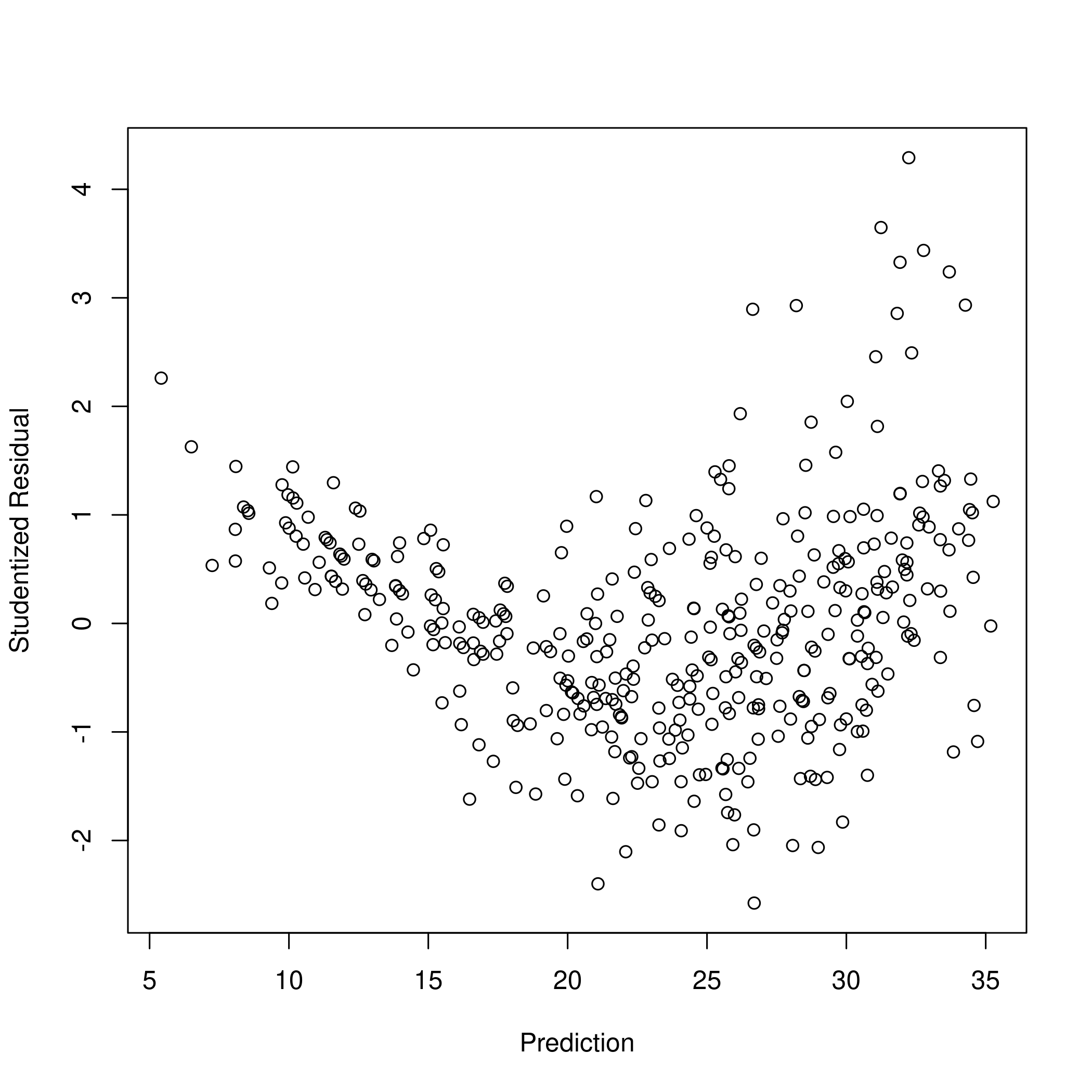
1# Predict and get the plot
2fitPlot <- noFactors %>% lm(mpg~.,data=.)
3# See residuals
4plot(xlab="Prediction",ylab="Studentized Residual",x=predict(fitPlot),y=rstudent(fitPlot))
1# Try a linear fit of studentized residuals
2par(mfrow=c(2,2))
3plot(lm(predict(fitPlot)~rstudent(fitPlot)))
Clearly the studentized residuals are nonlinear w.r.t the prediction. Also, some points are above the absolute value of \(3\) so they might be outliers, in keeping with the leverage plot.
(e) Interaction effects
We recall that x*y corresponds to x+y+x:y
1# View the correlation matrix
2cleanAuto %>% select(-name,-origin) %>% cor
 1##                     mpg  cylinders displacement horsepower     weight
 2## mpg           1.0000000 -0.7776175   -0.8051269 -0.7784268 -0.8322442
 3## cylinders    -0.7776175  1.0000000    0.9508233  0.8429834  0.8975273
 4## displacement -0.8051269  0.9508233    1.0000000  0.8972570  0.9329944
 5## horsepower   -0.7784268  0.8429834    0.8972570  1.0000000  0.8645377
 6## weight       -0.8322442  0.8975273    0.9329944  0.8645377  1.0000000
 7## acceleration  0.4233285 -0.5046834   -0.5438005 -0.6891955 -0.4168392
 8## year          0.5805410 -0.3456474   -0.3698552 -0.4163615 -0.3091199
 9##              acceleration       year
10## mpg             0.4233285  0.5805410
11## cylinders      -0.5046834 -0.3456474
12## displacement   -0.5438005 -0.3698552
13## horsepower     -0.6891955 -0.4163615
14## weight         -0.4168392 -0.3091199
15## acceleration    1.0000000  0.2903161
16## year            0.2903161  1.0000000
1summary(lm(mpg~weight*displacement*year,data=noFactors[(10:85),]))
 1##
 2## Call:
 3## lm(formula = mpg ~ weight * displacement * year, data = noFactors[(10:85),
 4##     ])
 5##
 6## Residuals:
 7##     Min      1Q  Median      3Q     Max
 8## -5.3020 -0.9055  0.0966  0.8912  3.7049
 9##
10## Coefficients:
11##                            Estimate Std. Error t value Pr(>|t|)
12## (Intercept)               3.961e+02  2.578e+02   1.537    0.129
13## weight                   -1.030e-01  1.008e-01  -1.021    0.311
14## displacement             -1.587e+00  1.308e+00  -1.213    0.229
15## year                     -4.889e+00  3.623e+00  -1.349    0.182
16## weight:displacement       3.926e-04  3.734e-04   1.051    0.297
17## weight:year               1.317e-03  1.418e-03   0.929    0.356
18## displacement:year         2.150e-02  1.846e-02   1.165    0.248
19## weight:displacement:year -5.287e-06  5.253e-06  -1.007    0.318
20##
21## Residual standard error: 1.8 on 68 degrees of freedom
22## Multiple R-squared:  0.922,  Adjusted R-squared:  0.914
23## F-statistic: 114.9 on 7 and 68 DF,  p-value: < 2.2e-16
1summary(lm(mpg~weight*displacement*year,data=noFactors))
 1##
 2## Call:
 3## lm(formula = mpg ~ weight * displacement * year, data = noFactors)
 4##
 5## Residuals:
 6##     Min      1Q  Median      3Q     Max
 7## -9.6093 -1.6472 -0.0531  1.2289 14.5604
 8##
 9## Coefficients:
10##                            Estimate Std. Error t value Pr(>|t|)
11## (Intercept)              -8.437e+01  3.128e+01  -2.697   0.0073 **
12## weight                    8.489e-03  1.322e-02   0.642   0.5212
13## displacement              3.434e-01  1.969e-01   1.744   0.0820 .
14## year                      1.828e+00  4.127e-01   4.430 1.23e-05 ***
15## weight:displacement      -6.589e-05  5.055e-05  -1.303   0.1932
16## weight:year              -2.433e-04  1.744e-04  -1.395   0.1638
17## displacement:year        -5.566e-03  2.674e-03  -2.082   0.0380 *
18## weight:displacement:year  1.144e-06  6.823e-07   1.677   0.0944 .
19## ---
20## Signif. codes:  0 '***' 0.001 '**' 0.01 '*' 0.05 '.' 0.1 ' ' 1
21##
22## Residual standard error: 2.951 on 384 degrees of freedom
23## Multiple R-squared:  0.8596, Adjusted R-squared:  0.8571
24## F-statistic:   336 on 7 and 384 DF,  p-value: < 2.2e-16
- Adding the interaction effects of the \(3\) most positive R value terms improves the existing prediction to be better than that obtained by considering all effects.
- We note that the best model is obtained by removing the range identified in chapter 2.
(f) Nonlinear transformations
1summary(lm(mpg~weight*displacement*year+I(year^2),data=noFactors[(10:85),]))
 1##
 2## Call:
 3## lm(formula = mpg ~ weight * displacement * year + I(year^2),
 4##     data = noFactors[(10:85), ])
 5##
 6## Residuals:
 7##     Min      1Q  Median      3Q     Max
 8## -5.1815 -0.8235  0.0144  1.0076  3.9420
 9##
10## Coefficients:
11##                            Estimate Std. Error t value Pr(>|t|)
12## (Intercept)              -4.205e+03  1.810e+03  -2.324   0.0232 *
13## weight                   -8.800e-02  9.709e-02  -0.906   0.3680
14## displacement             -1.030e+00  1.276e+00  -0.807   0.4225
15## year                      1.238e+02  5.026e+01   2.464   0.0163 *
16## I(year^2)                -9.000e-01  3.506e-01  -2.567   0.0125 *
17## weight:displacement       2.471e-04  3.634e-04   0.680   0.4988
18## weight:year               1.113e-03  1.365e-03   0.815   0.4177
19## displacement:year         1.368e-02  1.800e-02   0.760   0.4501
20## weight:displacement:year -3.254e-06  5.111e-06  -0.637   0.5264
21## ---
22## Signif. codes:  0 '***' 0.001 '**' 0.01 '*' 0.05 '.' 0.1 ' ' 1
23##
24## Residual standard error: 1.73 on 67 degrees of freedom
25## Multiple R-squared:  0.929,  Adjusted R-squared:  0.9205
26## F-statistic: 109.6 on 8 and 67 DF,  p-value: < 2.2e-16
1summary(lm(mpg~.-I(log(acceleration^2)),data=noFactors[(10:85),]))
 1##
 2## Call:
 3## lm(formula = mpg ~ . - I(log(acceleration^2)), data = noFactors[(10:85),
 4##     ])
 5##
 6## Residuals:
 7##    Min     1Q Median     3Q    Max
 8## -6.232 -1.470 -0.211  1.075  7.088
 9##
10## Coefficients:
11##                Estimate Std. Error t value Pr(>|t|)
12## (Intercept)  41.3787633 24.1208720   1.715   0.0907 .
13## cylinders     0.0863161  0.6112822   0.141   0.8881
14## displacement -0.0148491  0.0103249  -1.438   0.1549
15## horsepower   -0.0158500  0.0151259  -1.048   0.2984
16## weight       -0.0039125  0.0008546  -4.578 2.02e-05 ***
17## acceleration -0.1473786  0.1438220  -1.025   0.3091
18## year         -0.0378187  0.3380266  -0.112   0.9112
19## ---
20## Signif. codes:  0 '***' 0.001 '**' 0.01 '*' 0.05 '.' 0.1 ' ' 1
21##
22## Residual standard error: 2.262 on 69 degrees of freedom
23## Multiple R-squared:  0.8751, Adjusted R-squared:  0.8642
24## F-statistic: 80.55 on 6 and 69 DF,  p-value: < 2.2e-16
The best model I found was still the one without the non-linear transformation but with removed outliers and additional interaction effects of
displacement,=year= andweightA popular approach is to use a
logtransform for both the inputs and the outputs
1summary(lm(log(mpg)~.,data=noFactors[(10:85),]))
 1##
 2## Call:
 3## lm(formula = log(mpg) ~ ., data = noFactors[(10:85), ])
 4##
 5## Residuals:
 6##       Min        1Q    Median        3Q       Max
 7## -0.285805 -0.052358 -0.001456  0.066521  0.209739
 8##
 9## Coefficients:
10##                Estimate Std. Error t value Pr(>|t|)
11## (Intercept)   3.886e+00  1.028e+00   3.781 0.000328 ***
12## cylinders    -1.771e-02  2.604e-02  -0.680 0.498669
13## displacement -1.540e-04  4.399e-04  -0.350 0.727314
14## horsepower   -2.343e-03  6.444e-04  -3.636 0.000529 ***
15## weight       -1.960e-04  3.641e-05  -5.383 9.51e-07 ***
16## acceleration -1.525e-02  6.128e-03  -2.489 0.015224 *
17## year          4.138e-03  1.440e-02   0.287 0.774703
18## ---
19## Signif. codes:  0 '***' 0.001 '**' 0.01 '*' 0.05 '.' 0.1 ' ' 1
20##
21## Residual standard error: 0.09636 on 69 degrees of freedom
22## Multiple R-squared:  0.919,  Adjusted R-squared:  0.912
23## F-statistic: 130.5 on 6 and 69 DF,  p-value: < 2.2e-16
1summary(lm(log(mpg)~log(weight*displacement*year),data=noFactors[(10:85),]))
 1##
 2## Call:
 3## lm(formula = log(mpg) ~ log(weight * displacement * year), data = noFactors[(10:85),
 4##     ])
 5##
 6## Residuals:
 7##      Min       1Q   Median       3Q      Max
 8## -0.41121 -0.04107  0.01266  0.07791  0.21056
 9##
10## Coefficients:
11##                                   Estimate Std. Error t value Pr(>|t|)
12## (Intercept)                        8.91995    0.26467   33.70   <2e-16 ***
13## log(weight * displacement * year) -0.34250    0.01508  -22.71   <2e-16 ***
14## ---
15## Signif. codes:  0 '***' 0.001 '**' 0.01 '*' 0.05 '.' 0.1 ' ' 1
16##
17## Residual standard error: 0.1158 on 74 degrees of freedom
18## Multiple R-squared:  0.8745, Adjusted R-squared:  0.8728
19## F-statistic: 515.6 on 1 and 74 DF,  p-value: < 2.2e-16
Question 3.10 - Page 123
This question should be answered using the Carseats data set.
(a) Fit a multiple regression model to predict Sales using Price,
Urban, and US.
(b) Provide an interpretation of each coefficient in the model. Be careful—some of the variables in the model are qualitative!
(c) Write out the model in equation form, being careful to handle the qualitative variables properly.
(d) For which of the predictors can you reject the null hypothesis \(H_0:\beta_j=0\)?
(e) On the basis of your response to the previous question, fit a smaller model that only uses the predictors for which there is evidence of association with the outcome.
(f) How well do the models in (a) and (e) fit the data?
(g) Using the model from (e), obtain \(95%\) confidence intervals for the coefficient(s).
(h) Is there evidence of outliers or high leverage observations in the model from (e)?
Answer
Load the dataset (and clean it)
1cleanCarSeats <- na.omit(ISLR::Carseats)
Obtain summary statistics
1cleanCarSeats %>% sapply(unique) %>% sapply(length)
1##       Sales   CompPrice      Income Advertising  Population       Price
2##         336          73          98          28         275         101
3##   ShelveLoc         Age   Education       Urban          US
4##           3          56           9           2           2
1str(cleanCarSeats)
 1## 'data.frame':    400 obs. of  11 variables:
 2##  $ Sales      : num  9.5 11.22 10.06 7.4 4.15 ...
 3##  $ CompPrice  : num  138 111 113 117 141 124 115 136 132 132 ...
 4##  $ Income     : num  73 48 35 100 64 113 105 81 110 113 ...
 5##  $ Advertising: num  11 16 10 4 3 13 0 15 0 0 ...
 6##  $ Population : num  276 260 269 466 340 501 45 425 108 131 ...
 7##  $ Price      : num  120 83 80 97 128 72 108 120 124 124 ...
 8##  $ ShelveLoc  : Factor w/ 3 levels "Bad","Good","Medium": 1 2 3 3 1 1 3 2 3 3 ...
 9##  $ Age        : num  42 65 59 55 38 78 71 67 76 76 ...
10##  $ Education  : num  17 10 12 14 13 16 15 10 10 17 ...
11##  $ Urban      : Factor w/ 2 levels "No","Yes": 2 2 2 2 2 1 2 2 1 1 ...
12##  $ US         : Factor w/ 2 levels "No","Yes": 2 2 2 2 1 2 1 2 1 2 ...
1summary(cleanCarSeats)
 1##      Sales          CompPrice       Income        Advertising
 2##  Min.   : 0.000   Min.   : 77   Min.   : 21.00   Min.   : 0.000
 3##  1st Qu.: 5.390   1st Qu.:115   1st Qu.: 42.75   1st Qu.: 0.000
 4##  Median : 7.490   Median :125   Median : 69.00   Median : 5.000
 5##  Mean   : 7.496   Mean   :125   Mean   : 68.66   Mean   : 6.635
 6##  3rd Qu.: 9.320   3rd Qu.:135   3rd Qu.: 91.00   3rd Qu.:12.000
 7##  Max.   :16.270   Max.   :175   Max.   :120.00   Max.   :29.000
 8##    Population        Price        ShelveLoc        Age          Education
 9##  Min.   : 10.0   Min.   : 24.0   Bad   : 96   Min.   :25.00   Min.   :10.0
10##  1st Qu.:139.0   1st Qu.:100.0   Good  : 85   1st Qu.:39.75   1st Qu.:12.0
11##  Median :272.0   Median :117.0   Medium:219   Median :54.50   Median :14.0
12##  Mean   :264.8   Mean   :115.8                Mean   :53.32   Mean   :13.9
13##  3rd Qu.:398.5   3rd Qu.:131.0                3rd Qu.:66.00   3rd Qu.:16.0
14##  Max.   :509.0   Max.   :191.0                Max.   :80.00   Max.   :18.0
15##  Urban       US
16##  No :118   No :142
17##  Yes:282   Yes:258
18##
19##
20##
21##
We can see that:
- Urban, US and ShelveLoc are factors with 2,2 and 3 levels respectively
- Education has only 9 unique values so we might as well consider it to be a factor too if we need to
(a) Multiple Regression Model
Fit it to things
1summary(lm(Sales~.,data=cleanCarSeats))
 1##
 2## Call:
 3## lm(formula = Sales ~ ., data = cleanCarSeats)
 4##
 5## Residuals:
 6##     Min      1Q  Median      3Q     Max
 7## -2.8692 -0.6908  0.0211  0.6636  3.4115
 8##
 9## Coefficients:
10##                   Estimate Std. Error t value Pr(>|t|)
11## (Intercept)      5.6606231  0.6034487   9.380  < 2e-16 ***
12## CompPrice        0.0928153  0.0041477  22.378  < 2e-16 ***
13## Income           0.0158028  0.0018451   8.565 2.58e-16 ***
14## Advertising      0.1230951  0.0111237  11.066  < 2e-16 ***
15## Population       0.0002079  0.0003705   0.561    0.575
16## Price           -0.0953579  0.0026711 -35.700  < 2e-16 ***
17## ShelveLocGood    4.8501827  0.1531100  31.678  < 2e-16 ***
18## ShelveLocMedium  1.9567148  0.1261056  15.516  < 2e-16 ***
19## Age             -0.0460452  0.0031817 -14.472  < 2e-16 ***
20## Education       -0.0211018  0.0197205  -1.070    0.285
21## UrbanYes         0.1228864  0.1129761   1.088    0.277
22## USYes           -0.1840928  0.1498423  -1.229    0.220
23## ---
24## Signif. codes:  0 '***' 0.001 '**' 0.01 '*' 0.05 '.' 0.1 ' ' 1
25##
26## Residual standard error: 1.019 on 388 degrees of freedom
27## Multiple R-squared:  0.8734, Adjusted R-squared:  0.8698
28## F-statistic: 243.4 on 11 and 388 DF,  p-value: < 2.2e-16
1summary(lm(Sales~US*Price*Urban,data=cleanCarSeats))
 1##
 2## Call:
 3## lm(formula = Sales ~ US * Price * Urban, data = cleanCarSeats)
 4##
 5## Residuals:
 6##     Min      1Q  Median      3Q     Max
 7## -6.7952 -1.6659 -0.0984  1.6119  7.2433
 8##
 9## Coefficients:
10##                       Estimate Std. Error t value Pr(>|t|)
11## (Intercept)          13.456350   1.727210   7.791 6.03e-14 ***
12## USYes                 2.049051   2.322591   0.882    0.378
13## Price                -0.061657   0.014875  -4.145 4.17e-05 ***
14## UrbanYes             -0.651545   2.071401  -0.315    0.753
15## USYes:Price          -0.001567   0.019972  -0.078    0.937
16## USYes:UrbanYes       -1.122034   2.759662  -0.407    0.685
17## Price:UrbanYes        0.010793   0.017796   0.606    0.545
18## USYes:Price:UrbanYes  0.001288   0.023619   0.055    0.957
19## ---
20## Signif. codes:  0 '***' 0.001 '**' 0.01 '*' 0.05 '.' 0.1 ' ' 1
21##
22## Residual standard error: 2.473 on 392 degrees of freedom
23## Multiple R-squared:  0.2467, Adjusted R-squared:  0.2333
24## F-statistic: 18.34 on 7 and 392 DF,  p-value: < 2.2e-16
1summary(lm(Sales~US+Price+Urban,data=cleanCarSeats))
 1##
 2## Call:
 3## lm(formula = Sales ~ US + Price + Urban, data = cleanCarSeats)
 4##
 5## Residuals:
 6##     Min      1Q  Median      3Q     Max
 7## -6.9206 -1.6220 -0.0564  1.5786  7.0581
 8##
 9## Coefficients:
10##              Estimate Std. Error t value Pr(>|t|)
11## (Intercept) 13.043469   0.651012  20.036  < 2e-16 ***
12## USYes        1.200573   0.259042   4.635 4.86e-06 ***
13## Price       -0.054459   0.005242 -10.389  < 2e-16 ***
14## UrbanYes    -0.021916   0.271650  -0.081    0.936
15## ---
16## Signif. codes:  0 '***' 0.001 '**' 0.01 '*' 0.05 '.' 0.1 ' ' 1
17##
18## Residual standard error: 2.472 on 396 degrees of freedom
19## Multiple R-squared:  0.2393, Adjusted R-squared:  0.2335
20## F-statistic: 41.52 on 3 and 396 DF,  p-value: < 2.2e-16
(b) Interpret stuff
To interpret the data, we need to determine which of the models fits the
data best, we will use anova() to test this:
1lmCarSAll<-lm(Sales~.,data=cleanCarSeats)
2lmCarStimesPUU<-lm(Sales~US*Price*Urban,data=cleanCarSeats)
3lmCarSplusPUU<-lm(Sales~US+Price+Urban,data=cleanCarSeats)
4anova(lmCarSAll,lmCarStimesPUU,lmCarSplusPUU)
 1## Analysis of Variance Table
 2##
 3## Model 1: Sales ~ CompPrice + Income + Advertising + Population + Price +
 4##     ShelveLoc + Age + Education + Urban + US
 5## Model 2: Sales ~ US * Price * Urban
 6## Model 3: Sales ~ US + Price + Urban
 7##   Res.Df     RSS Df Sum of Sq        F    Pr(>F)
 8## 1    388  402.83
 9## 2    392 2397.10 -4  -1994.27 480.2082 < 2.2e-16 ***
10## 3    396 2420.83 -4    -23.73   5.7149 0.0001772 ***
11## ---
12## Signif. codes:  0 '***' 0.001 '**' 0.01 '*' 0.05 '.' 0.1 ' ' 1
1anova(lmCarStimesPUU,lmCarSplusPUU)
1## Analysis of Variance Table
2##
3## Model 1: Sales ~ US * Price * Urban
4## Model 2: Sales ~ US + Price + Urban
5##   Res.Df    RSS Df Sum of Sq      F Pr(>F)
6## 1    392 2397.1
7## 2    396 2420.8 -4   -23.734 0.9703 0.4236
Remember that it is not possible to use anova() unless the same
variables are present in all the models being tested, so it is
meaningless to use anova for lmCarSAll along with the others,
because we can’t change the interaction model to get only the main
effects.
- We note that due to the low value of the F-statistic and the non-zero value of the p-value we cannot disregard the null hypothesis, or in other words, the models are basically the same in terms of their performance.
This means that I would like to continue with the simpler model, since the increase in R squared is too small to account for dealing with the additional factors.
- We see immediately, that there is a positive correlation only with being in the US
- Increases in price and being in an urban area actually decrease the sales, which is not surprising since being in the an urban area is probably correlated to a higher price, which we can check immediately
1summary(lm(Price~Urban,data=cleanCarSeats))
 1##
 2## Call:
 3## lm(formula = Price ~ Urban, data = cleanCarSeats)
 4##
 5## Residuals:
 6##     Min      1Q  Median      3Q     Max
 7## -92.514 -15.514   1.205  14.595  74.486
 8##
 9## Coefficients:
10##             Estimate Std. Error t value Pr(>|t|)
11## (Intercept)  114.076      2.180  52.330   <2e-16 ***
12## UrbanYes       2.438      2.596   0.939    0.348
13## ---
14## Signif. codes:  0 '***' 0.001 '**' 0.01 '*' 0.05 '.' 0.1 ' ' 1
15##
16## Residual standard error: 23.68 on 398 degrees of freedom
17## Multiple R-squared:  0.002211,   Adjusted R-squared:  -0.0002965
18## F-statistic: 0.8817 on 1 and 398 DF,  p-value: 0.3483
We see that our assumption is validated. Being in an urban area has a low t-statistic for a positive increase on the slope
- Returning to our previous model, we note that there is a high value of
the p-value of the t-statistic for
Urbanbeing true, this means there isn’t a real relationship between being in an urban area and the sales. This makes intuitive sense as well
note t-test is essentially a linear model with one variable, that
is, if we want to find out if there is a relation between having a store
in an urban area, we could sum all the urban yes and divide by the
number of observations and compare that to the sum of all the urban no
divided by the number of observations which is essentially the t-test
again.
Priceis significant, and has an inverse relation with the sales, so we should keep that in mind
(c) In Equation Form:
\[ Sales=1.200573*USYes - 0.054459*Price - 0.021916*UrbanYes + 13.043469 \]
(e) Other models
- We know from our case-study on testing the full multiple linear
regression for
Salesthat there are definitely more important variables being ignored. However, we also know thatUrbanis not significant, so we can use a smaller model.
1lmCarSplusPU<-lm(Sales~US+Price, data=cleanCarSeats)
(f) Comparison of models
1summary(lmCarSplusPU)
 1##
 2## Call:
 3## lm(formula = Sales ~ US + Price, data = cleanCarSeats)
 4##
 5## Residuals:
 6##     Min      1Q  Median      3Q     Max
 7## -6.9269 -1.6286 -0.0574  1.5766  7.0515
 8##
 9## Coefficients:
10##             Estimate Std. Error t value Pr(>|t|)
11## (Intercept) 13.03079    0.63098  20.652  < 2e-16 ***
12## USYes        1.19964    0.25846   4.641 4.71e-06 ***
13## Price       -0.05448    0.00523 -10.416  < 2e-16 ***
14## ---
15## Signif. codes:  0 '***' 0.001 '**' 0.01 '*' 0.05 '.' 0.1 ' ' 1
16##
17## Residual standard error: 2.469 on 397 degrees of freedom
18## Multiple R-squared:  0.2393, Adjusted R-squared:  0.2354
19## F-statistic: 62.43 on 2 and 397 DF,  p-value: < 2.2e-16
1anova(lmCarSplusPUU,lmCarSplusPU)
1## Analysis of Variance Table
2##
3## Model 1: Sales ~ US + Price + Urban
4## Model 2: Sales ~ US + Price
5##   Res.Df    RSS Df Sum of Sq      F Pr(>F)
6## 1    396 2420.8
7## 2    397 2420.9 -1  -0.03979 0.0065 0.9357
As expected, the low value of the F statistic and the high p-value for
the anova() test asserts that the null hypothesis cannot be neglected,
thus there are no differences between the model with the insignificant
parameter, which is also seen in the R squared value, which is the
same for both models
(g) Confidence Intervals
1confint(lmCarSplusPU)
1##                   2.5 %      97.5 %
2## (Intercept) 11.79032020 14.27126531
3## USYes        0.69151957  1.70776632
4## Price       -0.06475984 -0.04419543
1confint(lmCarSplusPUU)
1##                   2.5 %      97.5 %
2## (Intercept) 11.76359670 14.32334118
3## USYes        0.69130419  1.70984121
4## Price       -0.06476419 -0.04415351
5## UrbanYes    -0.55597316  0.51214085
- ☐ Look into trying to plot this with
ggplot
(h) Outliers
- We will first check the leverage plots
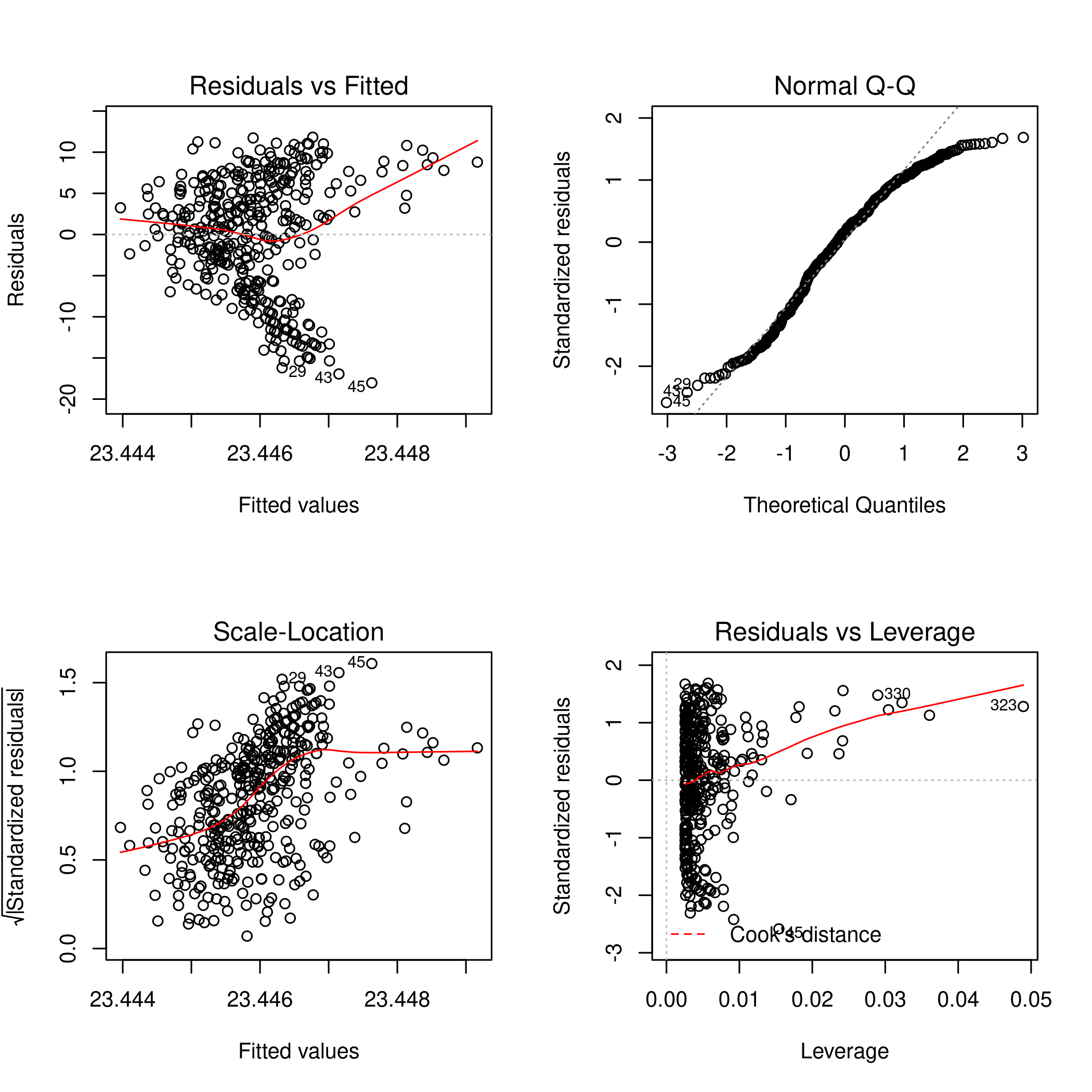
1par(mfrow=c(2,2))
2plot(lmCarSplusPU)
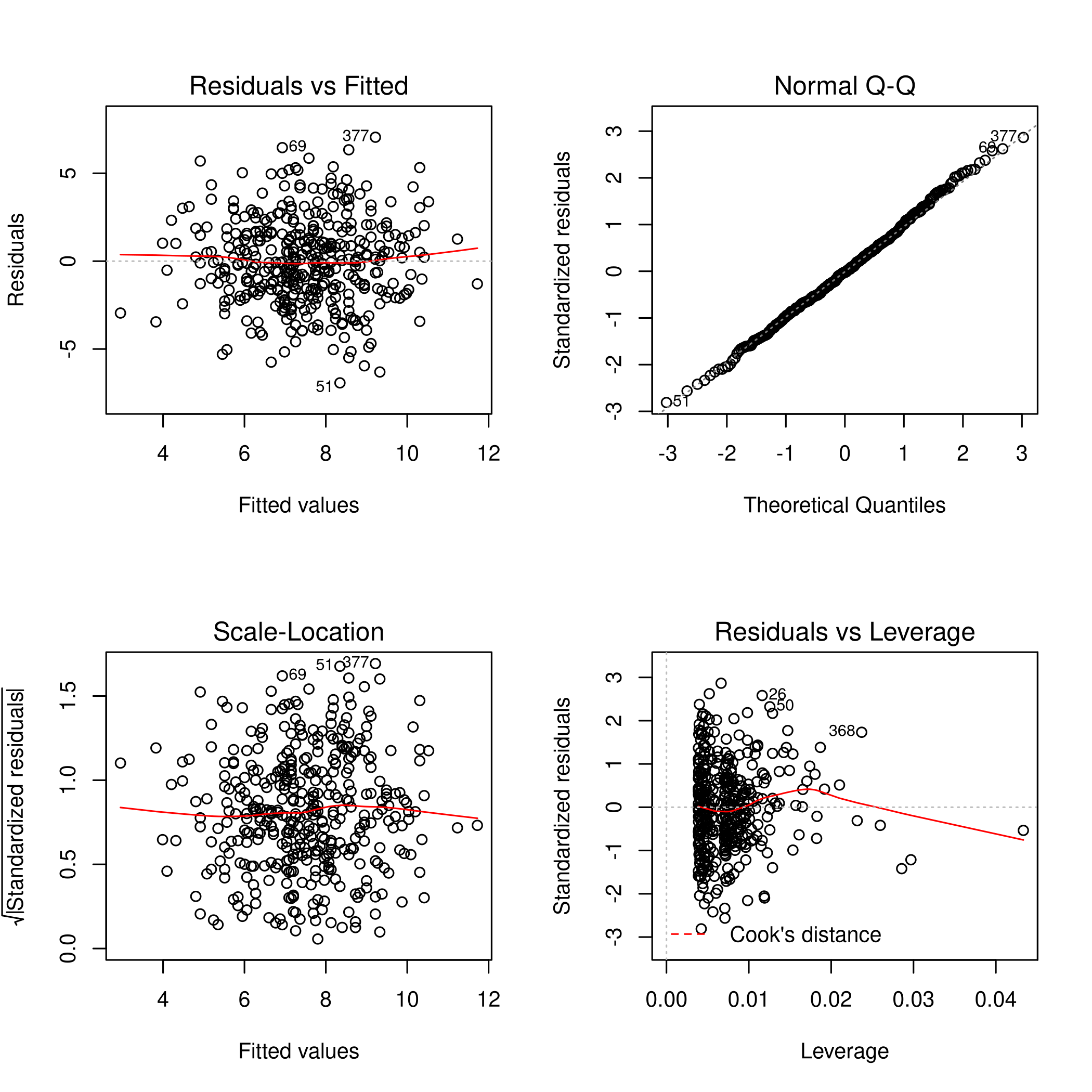
Figure 12: Leverage Plots
We can see there is a point with high leverage, but it has a low residual. In any case we should check further.
- Now we will check the studentized residuals to see if they are greater than 3
1# See residuals
2plot(xlab="Prediction",ylab="Studentized Residual",x=predict(lmCarSplusPU),y=rstudent(lmCarSplusPU))
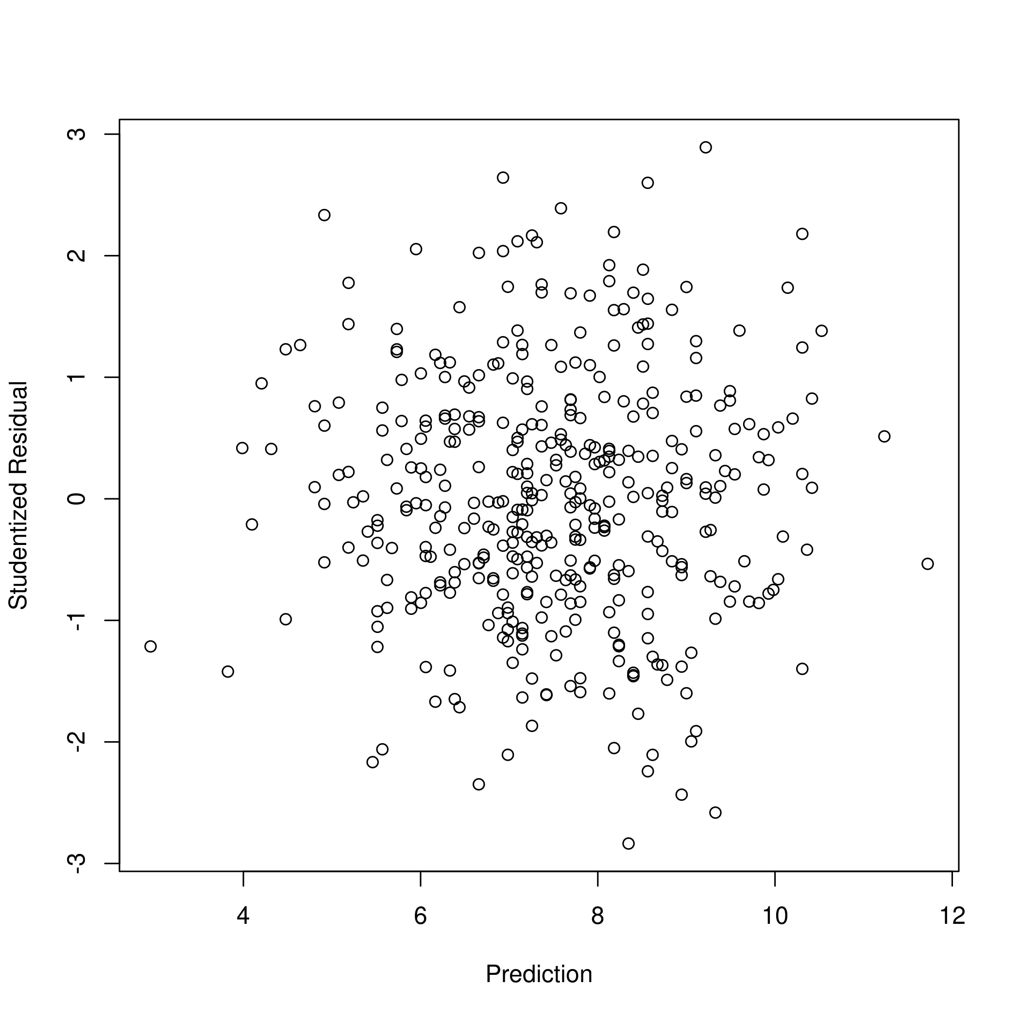
Figure 13: Studentized residuals
Thus I would say there are no outliers in our dataset, as none of our datapoints have an absolute studentized residual above 3.
James, G., Witten, D., Hastie, T., & Tibshirani, R. (2013). An Introduction to Statistical Learning: with Applications in R. Berlin, Germany: Springer Science & Business Media. ↩︎
![]()