
32 minutes
Written: 2020-02-17 15:28 +0000
ISLR :: Classification
Chapter IV - Classification
All the questions are as per the ISL seventh printing of the First edition 1.
Common Stuff
Here I’ll load things I will be using throughout, mostly libraries.
1libsUsed<-c("dplyr","ggplot2","tidyverse","ISLR","caret")
2invisible(lapply(libsUsed, library, character.only = TRUE))
Question 4.10 - Page 171
This question should be answered using the Weekly data set, which is
part of the ISLR package. This data is similar in nature to the Smarket
data from this chapter’s lab, except that it contains 1, 089 weekly
returns for 21 years, from the beginning of 1990 to the end of 2010.
(a) Produce some numerical and graphical summaries of the Weekly data. Do there appear to be any patterns?
(b) Use the full data set to perform a logistic regression with
Direction as the response and the five lag variables plus Volume as
predictors. Use the summary function to print the results. Do any of the
predictors appear to be statistically significant? If so, which ones?
(c) Compute the confusion matrix and overall fraction of correct predictions. Explain what the confusion matrix is telling you about the types of mistakes made by logistic regression.
(d) Now fit the logistic regression model using a training data period
from 1990 to 2008, with Lag2 as the only predictor. Compute the
confusion matrix and the overall fraction of correct predictions for the
held out data (that is, the data from 2009 and 2010).
(e) Repeat (d) using LDA.
(f) Repeat (d) using QDA.
(g) Repeat (d) using KNN with \(K = 1\).
(h) Which of these methods appears to provide the best results on this data?
(i) Experiment with different combinations of predictors, including possible transformations and interactions, for each of the methods. Report the variables, method, and associated confusion matrix that appears to provide the best results on the held out data. Note that you should also experiment with values for K in the KNN classifier.
Answer
We will need the data in a variable for ease of use.
1weeklyDat<-ISLR::Weekly
a) Summary Statistics
Text
Most of this segment relies heavily on usage of dplyr and especially
the %>% or pipe operator for readability. The use of the skimr
package2 might added more descriptive statistics, but is not
covered here.
Basic Summaries
1weeklyDat %>% str
 1# 'data.frame': 1089 obs. of  9 variables:
 2#  $ Year     : num  1990 1990 1990 1990 1990 1990 1990 1990 1990 1990 ...
 3#  $ Lag1     : num  0.816 -0.27 -2.576 3.514 0.712 ...
 4#  $ Lag2     : num  1.572 0.816 -0.27 -2.576 3.514 ...
 5#  $ Lag3     : num  -3.936 1.572 0.816 -0.27 -2.576 ...
 6#  $ Lag4     : num  -0.229 -3.936 1.572 0.816 -0.27 ...
 7#  $ Lag5     : num  -3.484 -0.229 -3.936 1.572 0.816 ...
 8#  $ Volume   : num  0.155 0.149 0.16 0.162 0.154 ...
 9#  $ Today    : num  -0.27 -2.576 3.514 0.712 1.178 ...
10#  $ Direction: Factor w/ 2 levels "Down","Up": 1 1 2 2 2 1 2 2 2 1 ...
We see that there is only one Factor, which makes sense.
1weeklyDat %>% summary
 1#       Year           Lag1               Lag2               Lag3
 2#  Min.   :1990   Min.   :-18.1950   Min.   :-18.1950   Min.   :-18.1950
 3#  1st Qu.:1995   1st Qu.: -1.1540   1st Qu.: -1.1540   1st Qu.: -1.1580
 4#  Median :2000   Median :  0.2410   Median :  0.2410   Median :  0.2410
 5#  Mean   :2000   Mean   :  0.1506   Mean   :  0.1511   Mean   :  0.1472
 6#  3rd Qu.:2005   3rd Qu.:  1.4050   3rd Qu.:  1.4090   3rd Qu.:  1.4090
 7#  Max.   :2010   Max.   : 12.0260   Max.   : 12.0260   Max.   : 12.0260
 8#       Lag4               Lag5              Volume            Today
 9#  Min.   :-18.1950   Min.   :-18.1950   Min.   :0.08747   Min.   :-18.1950
10#  1st Qu.: -1.1580   1st Qu.: -1.1660   1st Qu.:0.33202   1st Qu.: -1.1540
11#  Median :  0.2380   Median :  0.2340   Median :1.00268   Median :  0.2410
12#  Mean   :  0.1458   Mean   :  0.1399   Mean   :1.57462   Mean   :  0.1499
13#  3rd Qu.:  1.4090   3rd Qu.:  1.4050   3rd Qu.:2.05373   3rd Qu.:  1.4050
14#  Max.   : 12.0260   Max.   : 12.0260   Max.   :9.32821   Max.   : 12.0260
15#  Direction
16#  Down:484
17#  Up  :605
18#
19#
20#
21#
Unique Values
We might also want to know how many unique values are there in each column.
1weeklyDat %>% sapply(unique) %>% sapply(length)
1#      Year      Lag1      Lag2      Lag3      Lag4      Lag5    Volume     Today
2#        21      1004      1005      1005      1005      1005      1089      1003
3# Direction
4#         2
We note that year has disproportionately lower values, something to keep in mind while constructing models later.
Range
The range of each variable might be useful as well, but we have to ignore the factor.
1weeklyDat %>% subset(select=-c(Direction)) %>% sapply(range)
1#      Year    Lag1    Lag2    Lag3    Lag4    Lag5   Volume   Today
2# [1,] 1990 -18.195 -18.195 -18.195 -18.195 -18.195 0.087465 -18.195
3# [2,] 2010  12.026  12.026  12.026  12.026  12.026 9.328214  12.026
The most interesting thing about this is probably that the Lag
variables all have the same range, also something to be kept in mind
while applying transformations to the variable (if at all).
Mean and Std. Dev
By now we might have a pretty good idea of how this will look, but it is still worth seeing.
1weeklyDat %>% subset(select=-c(Direction)) %>% sapply(mean)
1#         Year         Lag1         Lag2         Lag3         Lag4         Lag5
2# 2000.0486685    0.1505849    0.1510790    0.1472048    0.1458182    0.1398926
3#       Volume        Today
4#    1.5746176    0.1498990
As expected, the Lag values have almost the same mean, what is a bit
interesting though, is that the Today variable has roughly the same
mean as the Lag variables.
1weeklyDat %>% subset(select=-c(Direction)) %>% sapply(sd)
1#     Year     Lag1     Lag2     Lag3     Lag4     Lag5   Volume    Today
2# 6.033182 2.357013 2.357254 2.360502 2.360279 2.361285 1.686636 2.356927
This is largely redundant in terms of new information.
Correlations
1weeklyDat %>% subset(select=-c(Direction)) %>% cor
 1#               Year         Lag1        Lag2        Lag3         Lag4
 2# Year    1.00000000 -0.032289274 -0.03339001 -0.03000649 -0.031127923
 3# Lag1   -0.03228927  1.000000000 -0.07485305  0.05863568 -0.071273876
 4# Lag2   -0.03339001 -0.074853051  1.00000000 -0.07572091  0.058381535
 5# Lag3   -0.03000649  0.058635682 -0.07572091  1.00000000 -0.075395865
 6# Lag4   -0.03112792 -0.071273876  0.05838153 -0.07539587  1.000000000
 7# Lag5   -0.03051910 -0.008183096 -0.07249948  0.06065717 -0.075675027
 8# Volume  0.84194162 -0.064951313 -0.08551314 -0.06928771 -0.061074617
 9# Today  -0.03245989 -0.075031842  0.05916672 -0.07124364 -0.007825873
10#                Lag5      Volume        Today
11# Year   -0.030519101  0.84194162 -0.032459894
12# Lag1   -0.008183096 -0.06495131 -0.075031842
13# Lag2   -0.072499482 -0.08551314  0.059166717
14# Lag3    0.060657175 -0.06928771 -0.071243639
15# Lag4   -0.075675027 -0.06107462 -0.007825873
16# Lag5    1.000000000 -0.05851741  0.011012698
17# Volume -0.058517414  1.00000000 -0.033077783
18# Today   0.011012698 -0.03307778  1.000000000
Useful though this is, it is kind of difficult to work with, in this form, so we might as well programmatic-ally remove strongly correlated data instead.
1# Uses caret
2corrCols=weeklyDat %>% subset(select=-c(Direction)) %>% cor %>% findCorrelation(cutoff=0.8)
3reducedDat<-weeklyDat[-c(corrCols)]
4reducedDat %>% summary
 1#       Year           Lag1               Lag2               Lag3
 2#  Min.   :1990   Min.   :-18.1950   Min.   :-18.1950   Min.   :-18.1950
 3#  1st Qu.:1995   1st Qu.: -1.1540   1st Qu.: -1.1540   1st Qu.: -1.1580
 4#  Median :2000   Median :  0.2410   Median :  0.2410   Median :  0.2410
 5#  Mean   :2000   Mean   :  0.1506   Mean   :  0.1511   Mean   :  0.1472
 6#  3rd Qu.:2005   3rd Qu.:  1.4050   3rd Qu.:  1.4090   3rd Qu.:  1.4090
 7#  Max.   :2010   Max.   : 12.0260   Max.   : 12.0260   Max.   : 12.0260
 8#       Lag4               Lag5              Today          Direction
 9#  Min.   :-18.1950   Min.   :-18.1950   Min.   :-18.1950   Down:484
10#  1st Qu.: -1.1580   1st Qu.: -1.1660   1st Qu.: -1.1540   Up  :605
11#  Median :  0.2380   Median :  0.2340   Median :  0.2410
12#  Mean   :  0.1458   Mean   :  0.1399   Mean   :  0.1499
13#  3rd Qu.:  1.4090   3rd Qu.:  1.4050   3rd Qu.:  1.4050
14#  Max.   : 12.0260   Max.   : 12.0260   Max.   : 12.0260
We can see that the Volume variable has been dropped, since it
evidently is strongly correlated with Year. This may or may not be a
useful insight, but it is good to keep in mind.
Visualization
We will be using the ggplot2 library throughout for this segment.
Lets start with some scatter plots in a one v/s all scheme, similar to the methodology described here.
1weeklyDat %>% subset(select=-c(Direction)) %>% gather(-Year,key="Variable", value="Value") %>% ggplot(aes(x=Value,y=Year)) +
2  geom_point() +
3  facet_wrap(~Variable) +
4  coord_flip()
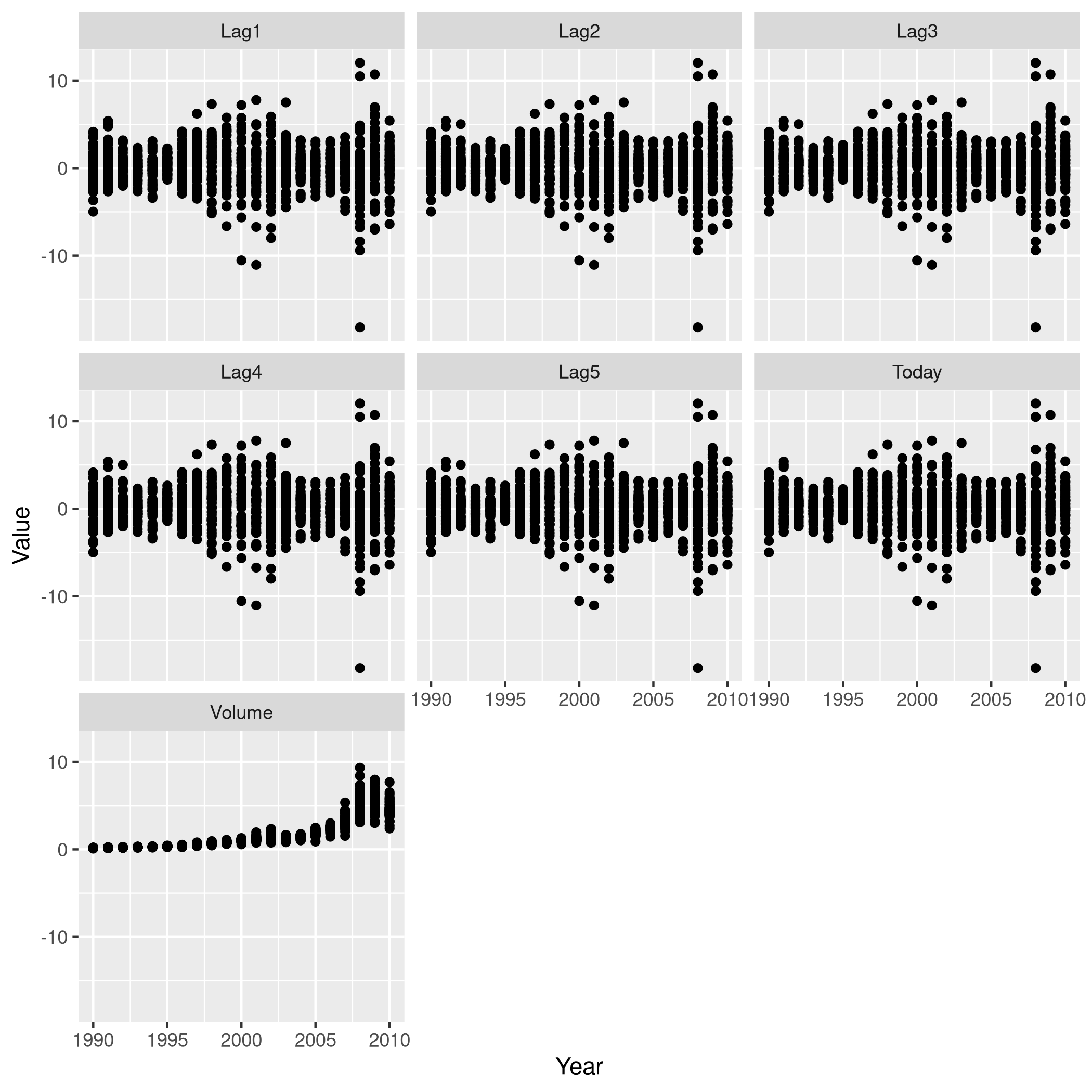
Figure 1: One v/s all for Direction
That didn’t really tell us much which we didn’t already get from the
cor() function, but we can go the whole hog and do this for every
variable since we don’t have that many in the first place..
1weeklyDat %>% subset(select=-c(Direction)) %>% pairs
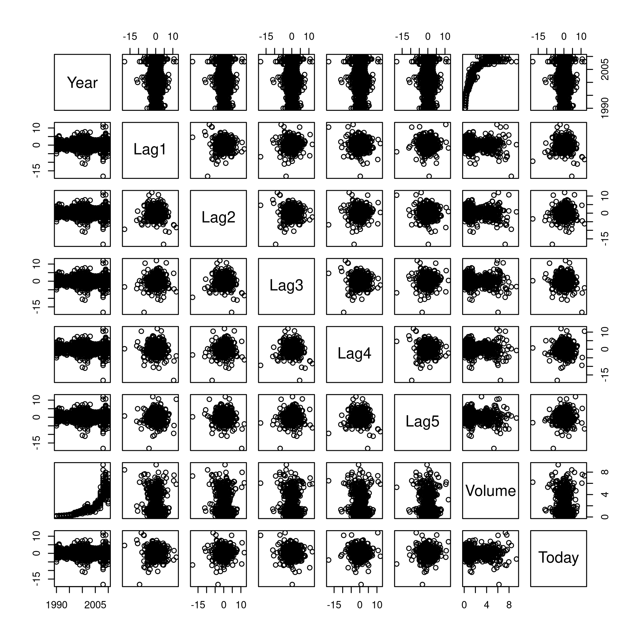
Figure 2: Pairs
This is not especially useful, and it is doubtful if more scatter-plots will help at all, so lets move on to box plots.
1weeklyDat %>% pivot_longer(-c(Direction,Volume,Today,Year),names_to="Lag",values_to="Value") %>% ggplot(aes(x=Direction,y=Value,fill=Lag)) +
2  geom_boxplot()
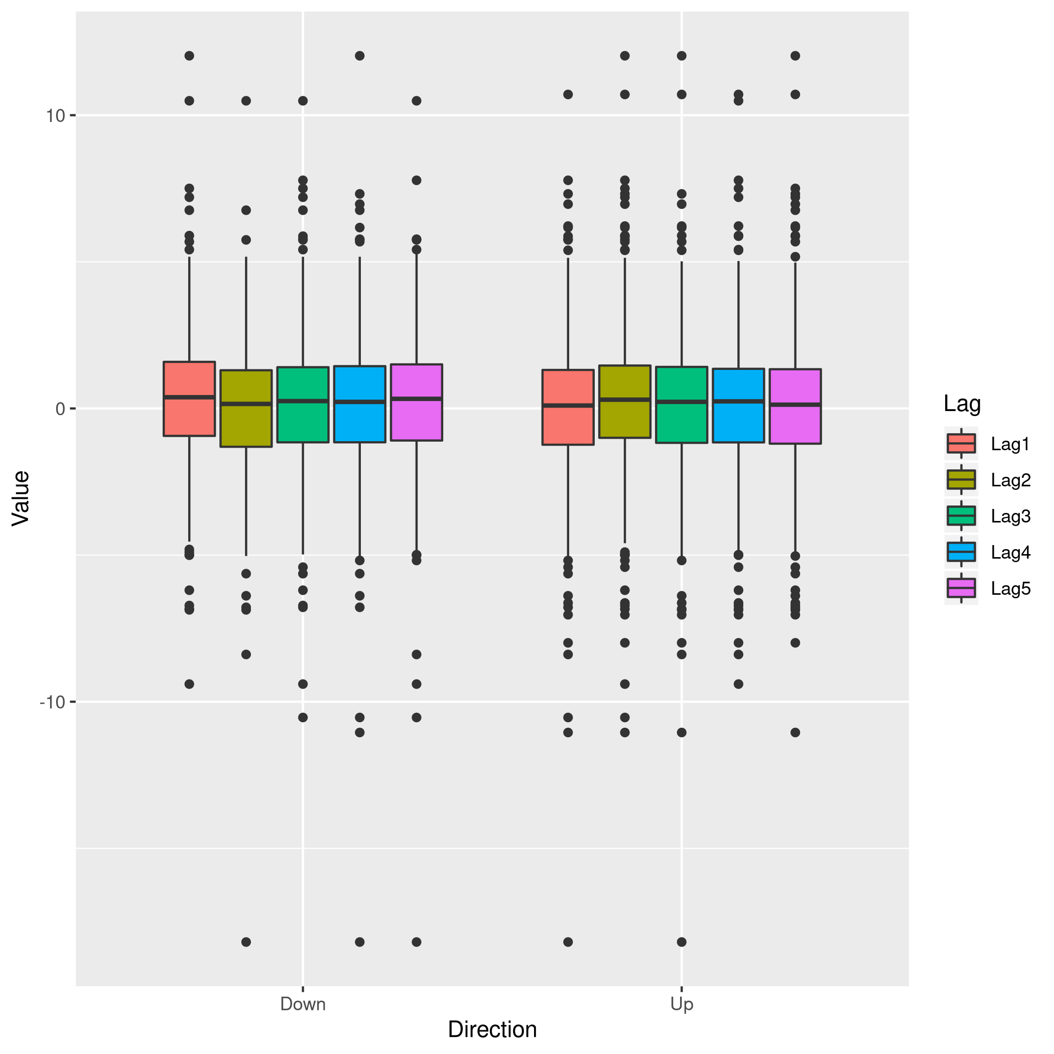
Figure 3: Box plots for Direction
1weeklyDat %>% pivot_longer(-c(Direction,Volume,Today,Year),names_to="Lag",values_to="Value") %>% ggplot(aes(x=Today,y=Value,fill=Lag)) +
2  geom_boxplot()
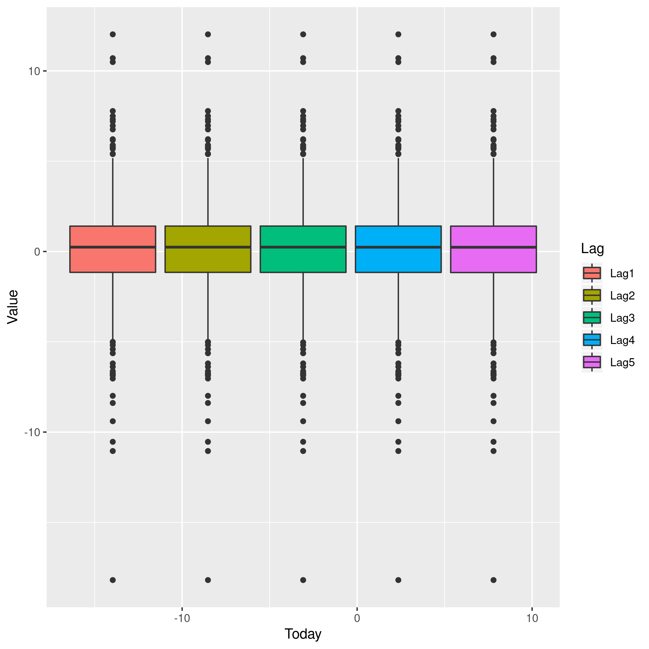
Figure 4: More box plots
1weeklyDat %>% pivot_longer(-c(Direction,Volume,Today,Year),names_to="Lag",values_to="Value") %>% ggplot(aes(x=Lag,y=Value,fill=Direction)) +
2  geom_boxplot()
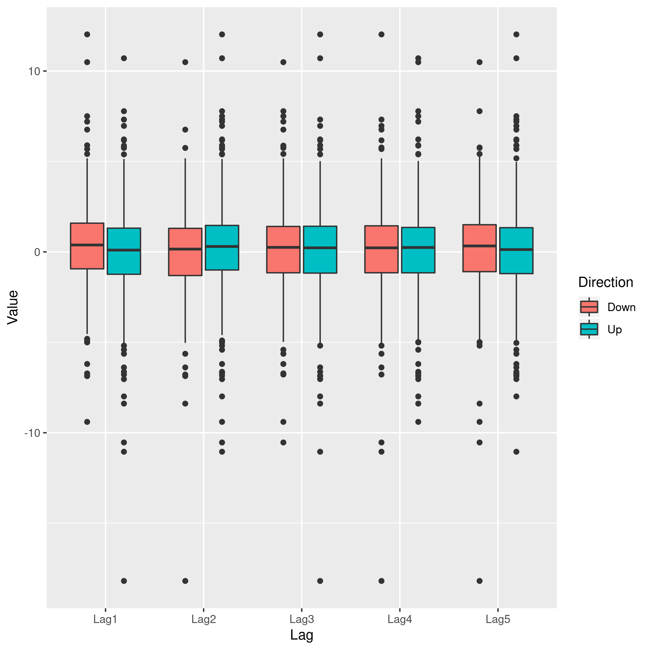
Figure 5: Lag v/s all
This does summarize our text analysis quite well. Importantly, it tells
us that the Today value is largely unrelated to the \(4\) Lag
variables.
A really good-looking box-plot is easy to get with the caret library:
1weeklyDat %>% subset(select=-c(Direction)) %>% featurePlot(
2            y = weeklyDat$Direction,
3            plot = "box",
4            # Pass in options to bwplot()
5            scales = list(y = list(relation="free"),
6                          x = list(rot = 90)),
7            auto.key = list(columns = 2))
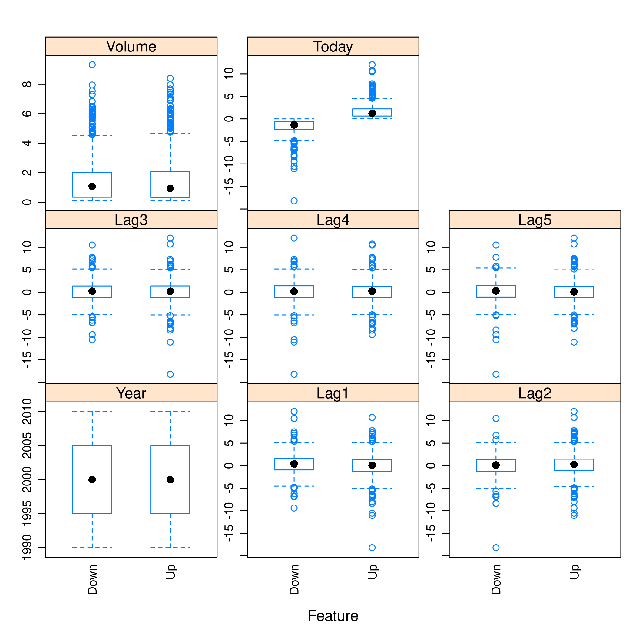
Figure 6: Plots with caret
We might want to visualize our correlation matrix as well.
1library(reshape2)
1#
2# Attaching package: 'reshape2'
1# The following object is masked from 'package:tidyr':
2#
3#     smiths
1weeklyDat %>% subset(select=-c(Direction)) %>% cor %>% melt %>% ggplot(aes(x=Var1,y=Var2,fill=value)) +
2  geom_tile()
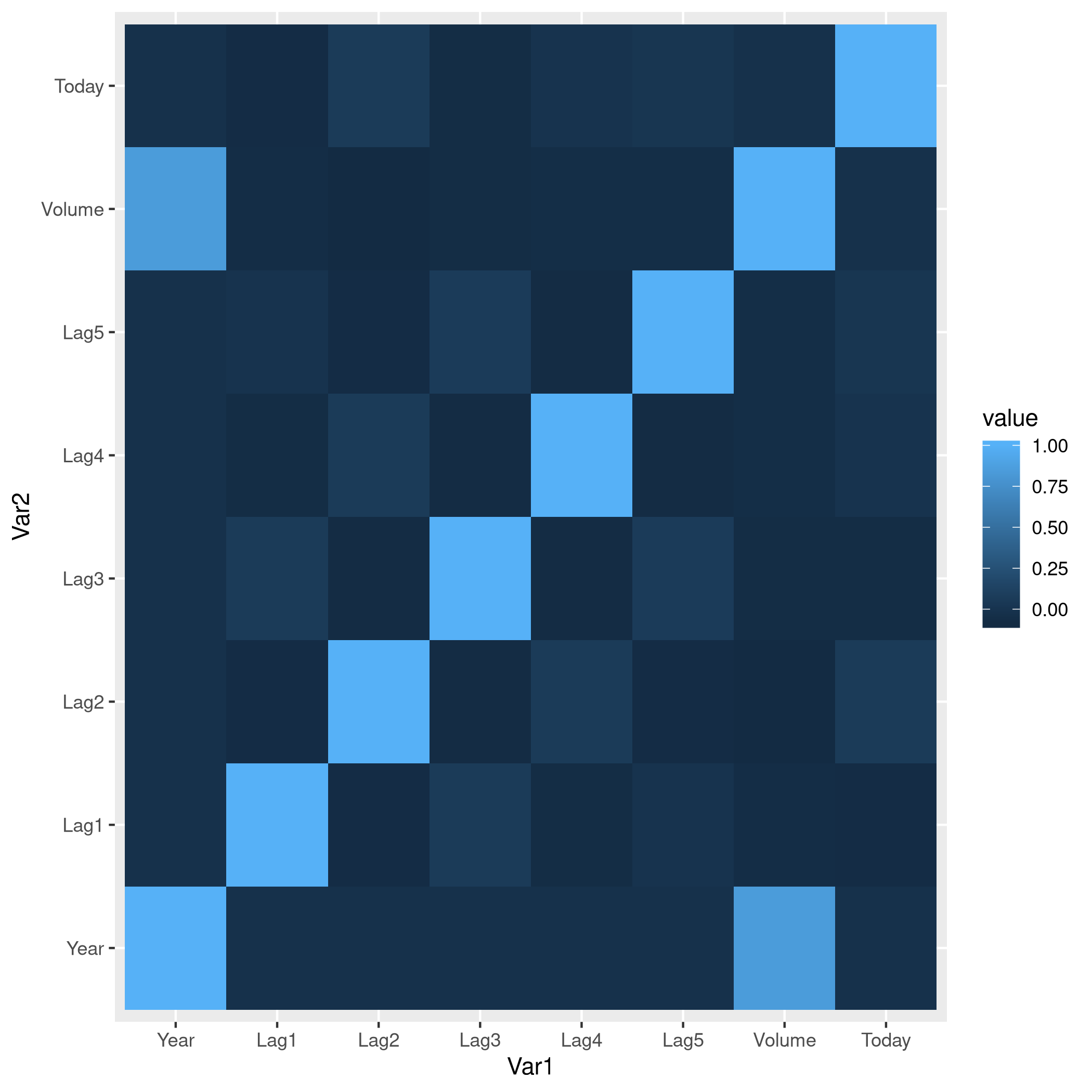
Figure 7: Heatmap of the correlation matrix
b) Logistic Regression - Predictor Significance
Lets start with the native glm function.
1glm.fit=glm(Direction~Lag1+Lag2+Lag3+Lag4+Lag5+Volume, data=weeklyDat, family=binomial)
2summary(glm.fit)
 1#
 2# Call:
 3# glm(formula = Direction ~ Lag1 + Lag2 + Lag3 + Lag4 + Lag5 +
 4#     Volume, family = binomial, data = weeklyDat)
 5#
 6# Deviance Residuals:
 7#     Min       1Q   Median       3Q      Max
 8# -1.6949  -1.2565   0.9913   1.0849   1.4579
 9#
10# Coefficients:
11#             Estimate Std. Error z value Pr(>|z|)
12# (Intercept)  0.26686    0.08593   3.106   0.0019 **
13# Lag1        -0.04127    0.02641  -1.563   0.1181
14# Lag2         0.05844    0.02686   2.175   0.0296 *
15# Lag3        -0.01606    0.02666  -0.602   0.5469
16# Lag4        -0.02779    0.02646  -1.050   0.2937
17# Lag5        -0.01447    0.02638  -0.549   0.5833
18# Volume      -0.02274    0.03690  -0.616   0.5377
19# ---
20# Signif. codes:  0 '***' 0.001 '**' 0.01 '*' 0.05 '.' 0.1 ' ' 1
21#
22# (Dispersion parameter for binomial family taken to be 1)
23#
24#     Null deviance: 1496.2  on 1088  degrees of freedom
25# Residual deviance: 1486.4  on 1082  degrees of freedom
26# AIC: 1500.4
27#
28# Number of Fisher Scoring iterations: 4
Evidently, only the Lag2 value is of statistical significance.
It is always of importance to figure out what numeric values R will assign to our factors, and it is best not to guess.
1contrasts(weeklyDat$Direction)
1#      Up
2# Down  0
3# Up    1
c) Confusion Matrix and Metrics
Essentially:
- Predict the response
- Create an output length vector
- Apply thresholding to obtain labels
1glm.probs = predict(glm.fit, type = "response")
2glm.pred = rep("Up",length(glm.probs))
3glm.pred[glm.probs<0.5]="Down"
4glm.pred=factor(glm.pred)
5confusionMatrix(glm.pred,weeklyDat$Direction)
 1# Confusion Matrix and Statistics
 2#
 3#           Reference
 4# Prediction Down  Up
 5#       Down   54  48
 6#       Up    430 557
 7#
 8#                Accuracy : 0.5611
 9#                  95% CI : (0.531, 0.5908)
10#     No Information Rate : 0.5556
11#     P-Value [Acc > NIR] : 0.369
12#
13#                   Kappa : 0.035
14#
15#  Mcnemar's Test P-Value : <2e-16
16#
17#             Sensitivity : 0.11157
18#             Specificity : 0.92066
19#          Pos Pred Value : 0.52941
20#          Neg Pred Value : 0.56434
21#              Prevalence : 0.44444
22#          Detection Rate : 0.04959
23#    Detection Prevalence : 0.09366
24#       Balanced Accuracy : 0.51612
25#
26#        'Positive' Class : Down
27#
- We have used the
confusionMatrixfunction fromcaret(documented here) instead of displaying the results withtableand then calculating precision, recall and the rest by hand.
d) Train Test Splits
Although we could have used the indices and passed it to glm as the
subset attribute, it is cleaner to just make subsets instead.
1weeklyVal<-weeklyDat %>% filter(Year>=2009)
2weeklyTrain<-weeklyDat %>% filter(Year<2009)
Now we can train a model on our training data.
1glm.fit=glm(Direction~Lag2,data=weeklyTrain,family=binomial)
2summary(glm.fit)
 1#
 2# Call:
 3# glm(formula = Direction ~ Lag2, family = binomial, data = weeklyTrain)
 4#
 5# Deviance Residuals:
 6#    Min      1Q  Median      3Q     Max
 7# -1.536  -1.264   1.021   1.091   1.368
 8#
 9# Coefficients:
10#             Estimate Std. Error z value Pr(>|z|)
11# (Intercept)  0.20326    0.06428   3.162  0.00157 **
12# Lag2         0.05810    0.02870   2.024  0.04298 *
13# ---
14# Signif. codes:  0 '***' 0.001 '**' 0.01 '*' 0.05 '.' 0.1 ' ' 1
15#
16# (Dispersion parameter for binomial family taken to be 1)
17#
18#     Null deviance: 1354.7  on 984  degrees of freedom
19# Residual deviance: 1350.5  on 983  degrees of freedom
20# AIC: 1354.5
21#
22# Number of Fisher Scoring iterations: 4
Having fit our model, we will test the predictions on our held out data.
1glm.probs = predict(glm.fit,weeklyVal, type = "response")
2glm.pred = rep("Up",length(glm.probs))
3glm.pred[glm.probs<0.5]="Down"
4glm.pred=factor(glm.pred)
5confusionMatrix(glm.pred,weeklyVal$Direction)
 1# Confusion Matrix and Statistics
 2#
 3#           Reference
 4# Prediction Down Up
 5#       Down    9  5
 6#       Up     34 56
 7#
 8#                Accuracy : 0.625
 9#                  95% CI : (0.5247, 0.718)
10#     No Information Rate : 0.5865
11#     P-Value [Acc > NIR] : 0.2439
12#
13#                   Kappa : 0.1414
14#
15#  Mcnemar's Test P-Value : 7.34e-06
16#
17#             Sensitivity : 0.20930
18#             Specificity : 0.91803
19#          Pos Pred Value : 0.64286
20#          Neg Pred Value : 0.62222
21#              Prevalence : 0.41346
22#          Detection Rate : 0.08654
23#    Detection Prevalence : 0.13462
24#       Balanced Accuracy : 0.56367
25#
26#        'Positive' Class : Down
27#
We really aren’t doing very well with this single variable model as is evident.
e) LDA models
At this stage we could use MASS to get the lda function, but it
would be better to just switch to using caret. Note that the caret
prediction is a label by default, so thresholding needs to be specified
differently if required.
1lda.fit=train(Direction~Lag2,data=weeklyTrain,method="lda")
2summary(lda.fit)
 1#             Length Class      Mode
 2# prior       2      -none-     numeric
 3# counts      2      -none-     numeric
 4# means       2      -none-     numeric
 5# scaling     1      -none-     numeric
 6# lev         2      -none-     character
 7# svd         1      -none-     numeric
 8# N           1      -none-     numeric
 9# call        3      -none-     call
10# xNames      1      -none-     character
11# problemType 1      -none-     character
12# tuneValue   1      data.frame list
13# obsLevels   2      -none-     character
14# param       0      -none-     list
1predict(lda.fit,weeklyVal) %>% confusionMatrix(weeklyVal$Direction)
 1# Confusion Matrix and Statistics
 2#
 3#           Reference
 4# Prediction Down Up
 5#       Down    9  5
 6#       Up     34 56
 7#
 8#                Accuracy : 0.625
 9#                  95% CI : (0.5247, 0.718)
10#     No Information Rate : 0.5865
11#     P-Value [Acc > NIR] : 0.2439
12#
13#                   Kappa : 0.1414
14#
15#  Mcnemar's Test P-Value : 7.34e-06
16#
17#             Sensitivity : 0.20930
18#             Specificity : 0.91803
19#          Pos Pred Value : 0.64286
20#          Neg Pred Value : 0.62222
21#              Prevalence : 0.41346
22#          Detection Rate : 0.08654
23#    Detection Prevalence : 0.13462
24#       Balanced Accuracy : 0.56367
25#
26#        'Positive' Class : Down
27#
f) QDA models
1qda.fit=train(Direction~Lag2,data=weeklyTrain,method="qda")
2summary(qda.fit)
 1#             Length Class      Mode
 2# prior       2      -none-     numeric
 3# counts      2      -none-     numeric
 4# means       2      -none-     numeric
 5# scaling     2      -none-     numeric
 6# ldet        2      -none-     numeric
 7# lev         2      -none-     character
 8# N           1      -none-     numeric
 9# call        3      -none-     call
10# xNames      1      -none-     character
11# problemType 1      -none-     character
12# tuneValue   1      data.frame list
13# obsLevels   2      -none-     character
14# param       0      -none-     list
1predict(qda.fit,weeklyVal) %>% confusionMatrix(weeklyVal$Direction)
 1# Confusion Matrix and Statistics
 2#
 3#           Reference
 4# Prediction Down Up
 5#       Down    0  0
 6#       Up     43 61
 7#
 8#                Accuracy : 0.5865
 9#                  95% CI : (0.4858, 0.6823)
10#     No Information Rate : 0.5865
11#     P-Value [Acc > NIR] : 0.5419
12#
13#                   Kappa : 0
14#
15#  Mcnemar's Test P-Value : 1.504e-10
16#
17#             Sensitivity : 0.0000
18#             Specificity : 1.0000
19#          Pos Pred Value :    NaN
20#          Neg Pred Value : 0.5865
21#              Prevalence : 0.4135
22#          Detection Rate : 0.0000
23#    Detection Prevalence : 0.0000
24#       Balanced Accuracy : 0.5000
25#
26#        'Positive' Class : Down
27#
This is quite possibly the worst of the lot. As is evident, the model
just predicts Up no matter what.
g) KNN
caret tends to over-zealously retrain models and find the best
possible parameters. In this case that is annoying and redundant so we
will use the class library. We should really scale our data before
using KNN though.
1library(class)
2set.seed(1)
3knn.pred=knn(as.matrix(weeklyTrain$Lag2),as.matrix(weeklyVal$Lag2),weeklyTrain$Direction,k=1)
4confusionMatrix(knn.pred,weeklyVal$Direction)
 1# Confusion Matrix and Statistics
 2#
 3#           Reference
 4# Prediction Down Up
 5#       Down   21 30
 6#       Up     22 31
 7#
 8#                Accuracy : 0.5
 9#                  95% CI : (0.4003, 0.5997)
10#     No Information Rate : 0.5865
11#     P-Value [Acc > NIR] : 0.9700
12#
13#                   Kappa : -0.0033
14#
15#  Mcnemar's Test P-Value : 0.3317
16#
17#             Sensitivity : 0.4884
18#             Specificity : 0.5082
19#          Pos Pred Value : 0.4118
20#          Neg Pred Value : 0.5849
21#              Prevalence : 0.4135
22#          Detection Rate : 0.2019
23#    Detection Prevalence : 0.4904
24#       Balanced Accuracy : 0.4983
25#
26#        'Positive' Class : Down
27#
Clearly this model is not doing very well.
h) Model Selection
We will first get the ROC curves.
1library(pROC)
1# Type 'citation("pROC")' for a citation.
1#
2# Attaching package: 'pROC'
1# The following objects are masked from 'package:stats':
2#
3#     cov, smooth, var
1knnROC<-roc(predictor=as.numeric(knn.pred),response=weeklyVal$Direction,levels=rev(levels(weeklyVal$Direction)))
1# Setting direction: controls < cases
1logiROC<-roc(predictor=as.numeric(predict(glm.fit,weeklyVal)),response=weeklyVal$Direction)
1# Setting levels: control = Down, case = Up
1# Setting direction: controls > cases
1ldaROC<-roc(predictor=as.numeric(predict(lda.fit,weeklyVal)),response=weeklyVal$Direction)
1# Setting levels: control = Down, case = Up
1# Setting direction: controls < cases
1qdaROC<-roc(predictor=as.numeric(predict(qda.fit,weeklyVal)),response=weeklyVal$Direction)
1# Setting levels: control = Down, case = Up
2# Setting direction: controls < cases
Now to plot them.
1ggroc(list(KNN=knnROC,Logistic=logiROC,LDA=ldaROC,QDA=qdaROC))
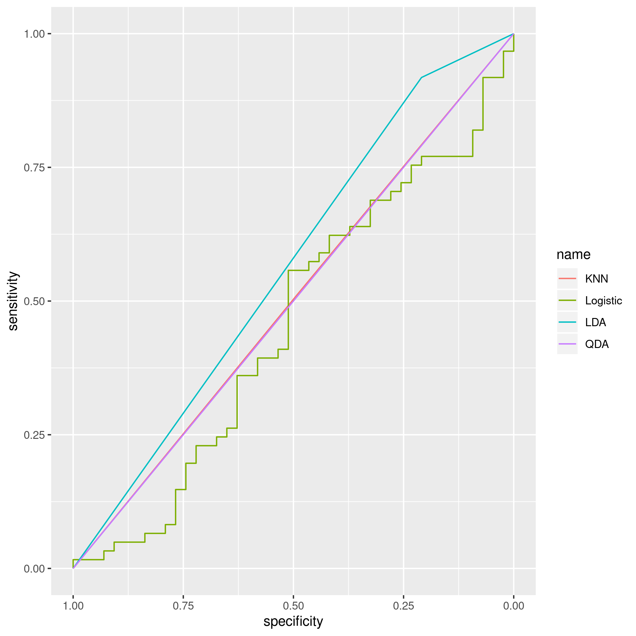
Figure 8: ROC curves for Weekly data
To compare models with caret it is easy to refit the logistic and knn
models in the caret formulation.
1knnCaret=train(Direction~Lag2,data=weeklyTrain,method="knn")
However, the KNN model is the best parameter model.
1resmod <- resamples(list(lda=lda.fit, qda=qda.fit, KNN=knnCaret))
2summary(resmod)
 1#
 2# Call:
 3# summary.resamples(object = resmod)
 4#
 5# Models: lda, qda, KNN
 6# Number of resamples: 25
 7#
 8# Accuracy
 9#          Min.   1st Qu.    Median      Mean   3rd Qu.      Max. NA's
10# lda 0.5043228 0.5344353 0.5529101 0.5500861 0.5683060 0.5846995    0
11# qda 0.5044248 0.5204360 0.5307263 0.5326785 0.5462428 0.5777778    0
12# KNN 0.4472222 0.5082873 0.5240642 0.5168327 0.5302198 0.5485714    0
13#
14# Kappa
15#            Min.      1st Qu.      Median         Mean    3rd Qu.       Max.
16# lda -0.02618939 -0.003638168 0.005796908  0.007801904 0.01635328 0.05431238
17# qda -0.06383592 -0.005606123 0.000000000 -0.003229697 0.00000000 0.03606344
18# KNN -0.11297539  0.004168597 0.024774647  0.016171229 0.04456142 0.07724439
19#     NA's
20# lda    0
21# qda    0
22# KNN    0
1bwplot(resmod)
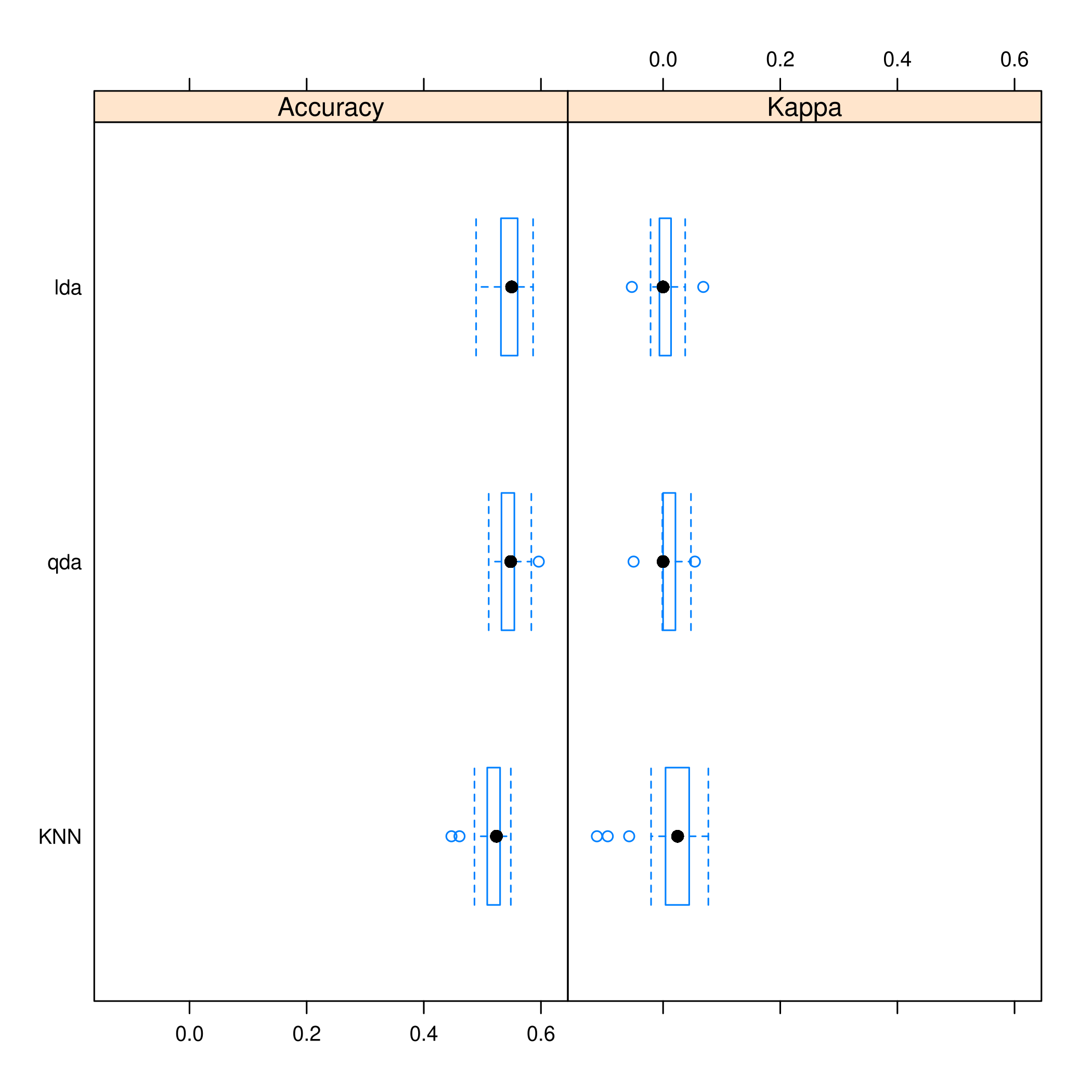
Figure 9: Caret plots for comparison
1dotplot(resmod)
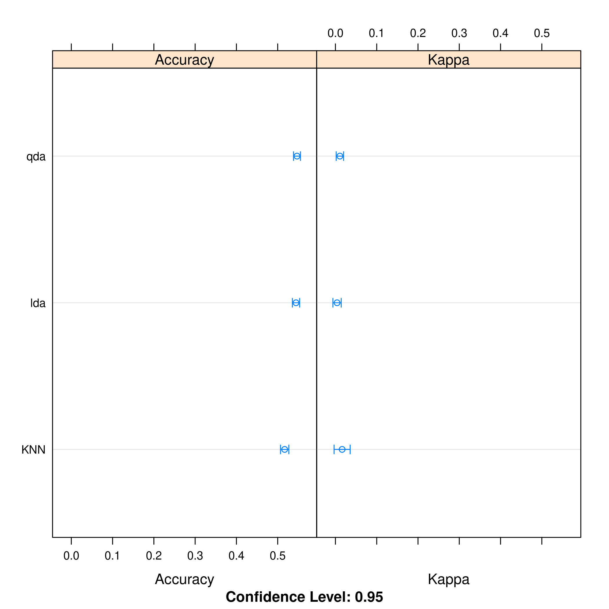
Kappa or Cohen’s Kappa is essentially classification accuracy, normalized at the baseline of random chance. It is a more useful measure to use on problems that have imbalanced classes. There’s more on model selection here.
i) Further Tuning
Do note the caret
defaults.
1fitControl <- trainControl(# 10-fold CV
2                           method = "repeatedcv",
3                           number = 10,
4                           # repeated ten times
5                           repeats = 10)
Logistic
1glm2.fit=glm(Direction~Lag1+Lag2+Lag3+Lag4+Lag5+Volume, data=weeklyDat, family=binomial)
2
3glm2.probs = predict(glm2.fit,weeklyVal, type = "response")
4glm2.pred = rep("Up",length(glm2.probs))
5glm2.pred[glm2.probs<0.5]="Down"
6glm2.pred=factor(glm2.pred)
7confusionMatrix(glm2.pred,weeklyVal$Direction)
 1# Confusion Matrix and Statistics
 2#
 3#           Reference
 4# Prediction Down Up
 5#       Down   17 13
 6#       Up     26 48
 7#
 8#                Accuracy : 0.625
 9#                  95% CI : (0.5247, 0.718)
10#     No Information Rate : 0.5865
11#     P-Value [Acc > NIR] : 0.24395
12#
13#                   Kappa : 0.1907
14#
15#  Mcnemar's Test P-Value : 0.05466
16#
17#             Sensitivity : 0.3953
18#             Specificity : 0.7869
19#          Pos Pred Value : 0.5667
20#          Neg Pred Value : 0.6486
21#              Prevalence : 0.4135
22#          Detection Rate : 0.1635
23#    Detection Prevalence : 0.2885
24#       Balanced Accuracy : 0.5911
25#
26#        'Positive' Class : Down
27#
QDA
1qdaCaret=train(Direction~Lag2+Lag4,data=weeklyTrain,method="qda",trainControl=fitControl)
1summary(qdaCaret)
 1#             Length Class      Mode
 2# prior       2      -none-     numeric
 3# counts      2      -none-     numeric
 4# means       4      -none-     numeric
 5# scaling     8      -none-     numeric
 6# ldet        2      -none-     numeric
 7# lev         2      -none-     character
 8# N           1      -none-     numeric
 9# call        4      -none-     call
10# xNames      2      -none-     character
11# problemType 1      -none-     character
12# tuneValue   1      data.frame list
13# obsLevels   2      -none-     character
14# param       1      -none-     list
1predict(qdaCaret,weeklyVal) %>% confusionMatrix(weeklyVal$Direction)
 1# Confusion Matrix and Statistics
 2#
 3#           Reference
 4# Prediction Down Up
 5#       Down    9 14
 6#       Up     34 47
 7#
 8#                Accuracy : 0.5385
 9#                  95% CI : (0.438, 0.6367)
10#     No Information Rate : 0.5865
11#     P-Value [Acc > NIR] : 0.863079
12#
13#                   Kappa : -0.0217
14#
15#  Mcnemar's Test P-Value : 0.006099
16#
17#             Sensitivity : 0.20930
18#             Specificity : 0.77049
19#          Pos Pred Value : 0.39130
20#          Neg Pred Value : 0.58025
21#              Prevalence : 0.41346
22#          Detection Rate : 0.08654
23#    Detection Prevalence : 0.22115
24#       Balanced Accuracy : 0.48990
25#
26#        'Positive' Class : Down
27#
LDA
1ldaCaret=train(Direction~Lag2+Lag1+Year,data=weeklyTrain,method="lda",trainControl=fitControl)
1summary(ldaCaret)
 1#             Length Class      Mode
 2# prior       2      -none-     numeric
 3# counts      2      -none-     numeric
 4# means       6      -none-     numeric
 5# scaling     3      -none-     numeric
 6# lev         2      -none-     character
 7# svd         1      -none-     numeric
 8# N           1      -none-     numeric
 9# call        4      -none-     call
10# xNames      3      -none-     character
11# problemType 1      -none-     character
12# tuneValue   1      data.frame list
13# obsLevels   2      -none-     character
14# param       1      -none-     list
1predict(ldaCaret,weeklyVal) %>% confusionMatrix(weeklyVal$Direction)
 1# Confusion Matrix and Statistics
 2#
 3#           Reference
 4# Prediction Down Up
 5#       Down   20 19
 6#       Up     23 42
 7#
 8#                Accuracy : 0.5962
 9#                  95% CI : (0.4954, 0.6913)
10#     No Information Rate : 0.5865
11#     P-Value [Acc > NIR] : 0.4626
12#
13#                   Kappa : 0.1558
14#
15#  Mcnemar's Test P-Value : 0.6434
16#
17#             Sensitivity : 0.4651
18#             Specificity : 0.6885
19#          Pos Pred Value : 0.5128
20#          Neg Pred Value : 0.6462
21#              Prevalence : 0.4135
22#          Detection Rate : 0.1923
23#    Detection Prevalence : 0.3750
24#       Balanced Accuracy : 0.5768
25#
26#        'Positive' Class : Down
27#
KNN
Honestly, again, this should be scaled. Plot KNN with the best
parameters.
1plot(knnCaret)
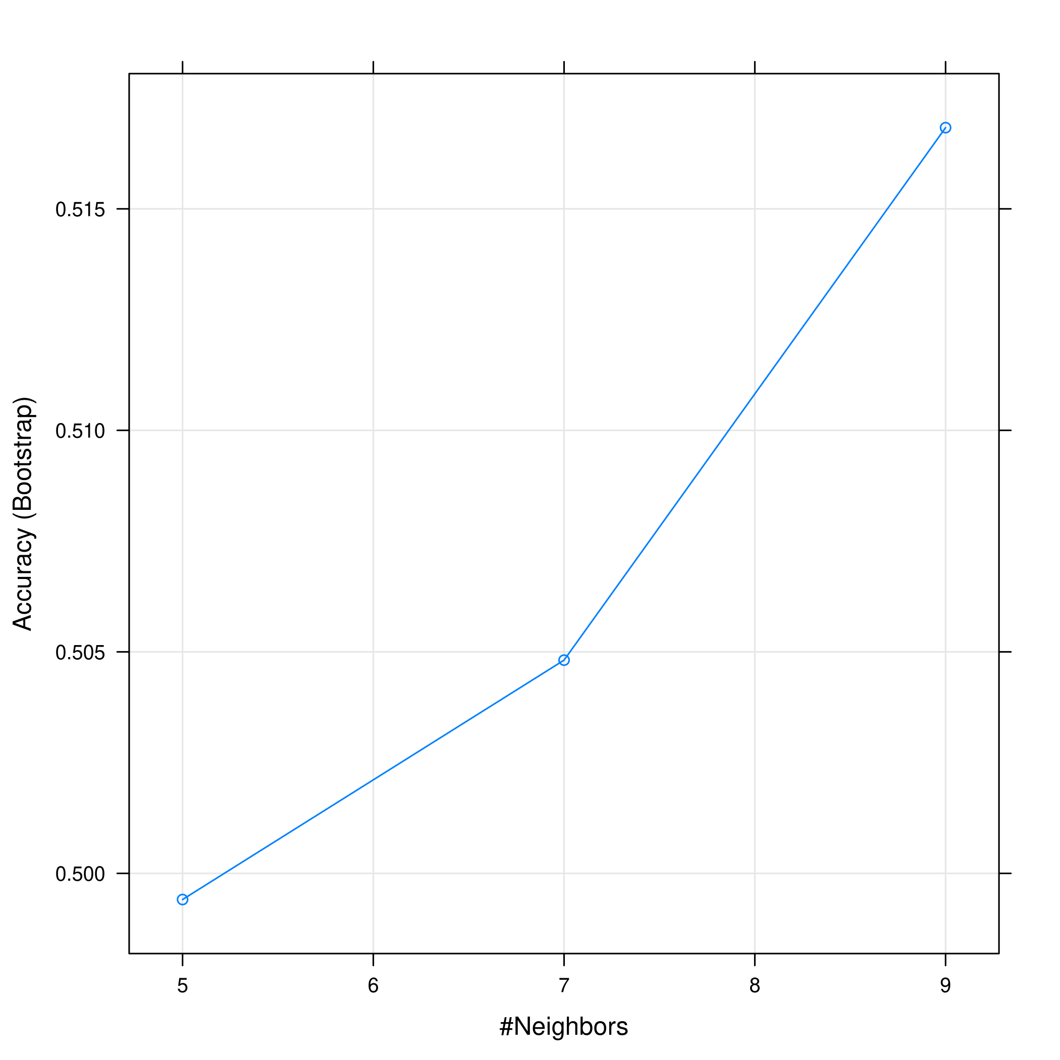
Figure 10: KNN statistics
Evidently, the accuracy increases with an increase in the number of neighbors considered.
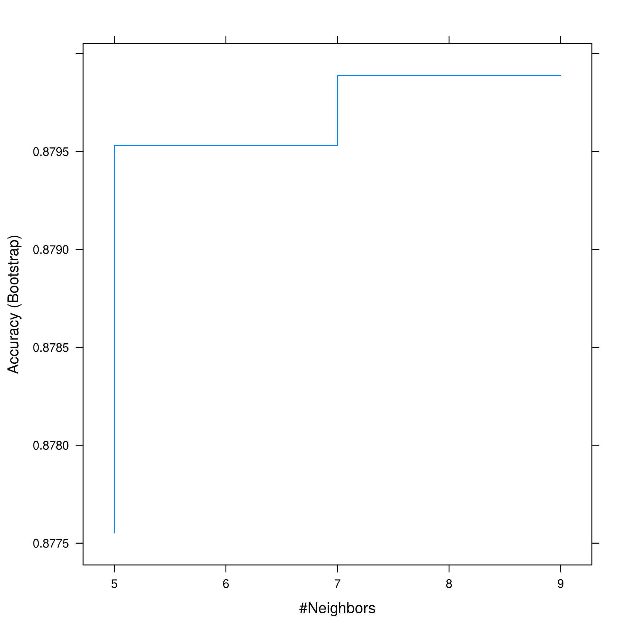
1plot(knnCaret, print.thres = 0.5, type="S")
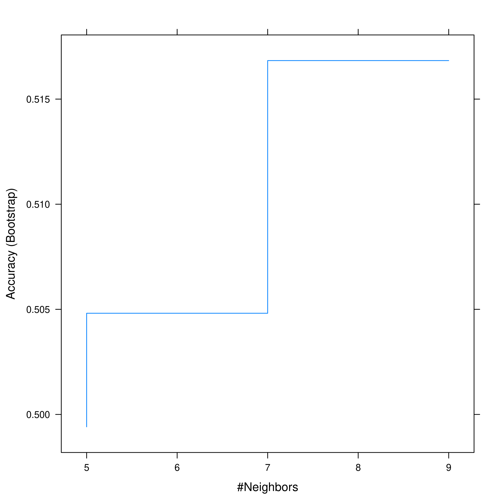
Figure 11: Visualizing thresholds for KNN
However this shows that we don’t actually get much of an increase in accuracy anyway.
Question 4.11 - Pages 171-172
In this problem, you will develop a model to predict whether a given car gets high or low gas mileage based on the Auto data set.
(a) Create a binary variable, mpg01 , that contains a 1 if mpg
contains a value above its median, and a 0 if mpg contains a value below
its median. You can compute the median using the median() function.
Note you may find it helpful to use the data.frame() function to
create a single data set containing both mpg01 and the other Auto
variables.
(b) Explore the data graphically in order to investigate the
association between mpg01 and the other features. Which of the other
features seem most likely to be useful in predicting mpg01 ?
Scatter-plots and boxplots may be useful tools to answer this question.
Describe your findings.
(c) Split the data into a training set and a test set.
(d) Perform LDA on the training data in order to predict mpg01 using
the variables that seemed most associated with mpg01 in (b). What is
the test error of the model obtained?
(e) Perform QDA on the training data in order to predict mpg01 using
the variables that seemed most associated with mpg01 in (b). What is
the test error of the model obtained?
(f) Perform logistic regression on the training data in order to
predict mpg01 using the variables that seemed most associated with
mpg01 in (b). What is the test error of the model obtained?
(g) Perform KNN on the training data, with several values of \(K\), in
order to predict mpg01 . Use only the variables that seemed most
associated with mpg01 in (b). What test errors do you obtain? Which
value of \(K\) seems to perform the best on this data set?
Answer
1autoDat<-ISLR::Auto
a) Binary Variable
1autoDat$mpg %>% sort() %>% median()
1# [1] 22.75
Now we can get a new variable from that.
1newDat=autoDat
2newDat$mpg01 <- ifelse(autoDat$mpg<autoDat$mpg %>% sort() %>% median(),0,1) %>% factor()
Note that the ifelse command takes a truthy function, value when
false, value when true, but does not return a factor automatically so we
piped it to factor to ensure it is factorial.
b) Visual Exploration
Some box-plots:
1newDat %>% pivot_longer(-c(mpg01,name),names_to="Params",values_to="Value") %>% ggplot(aes(x=mpg01,y=Value)) +
2  geom_boxplot() +
3  facet_wrap(~ Params, scales = "free_y")
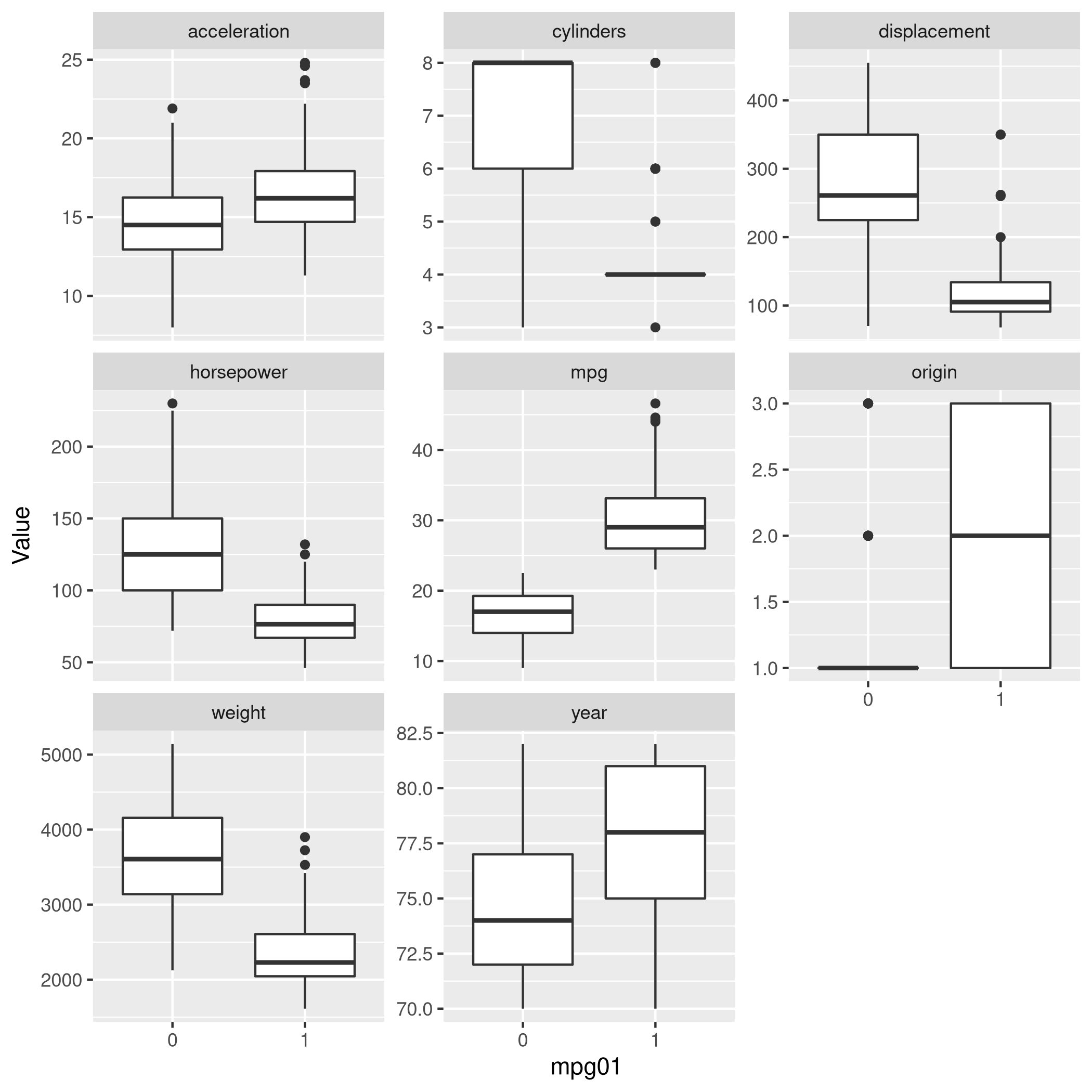
Figure 12: Box plots
With some scatter plots as well:
1newDat %>% pivot_longer(-c(mpg01,name,weight),names_to="Params",values_to="Value") %>% ggplot(aes(x=weight,y=Value,color=mpg01)) +
2  geom_point() +
3  facet_wrap(~ Params, scales = "free_y")
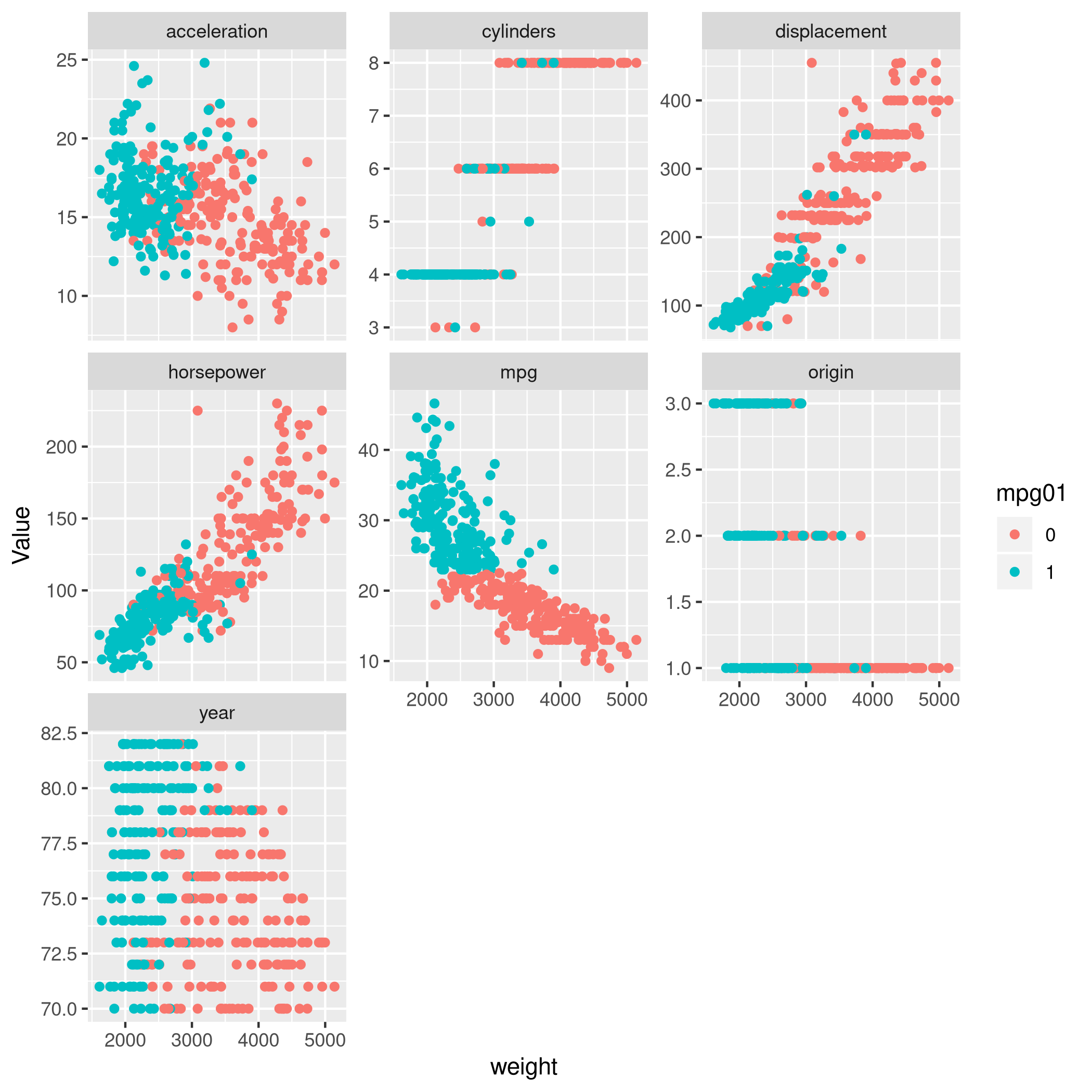
Figure 13: Scatter plots
Clearly, origin, year and cylinder are essentially not very
relevant numerically for the regression lines and confidence intervals.
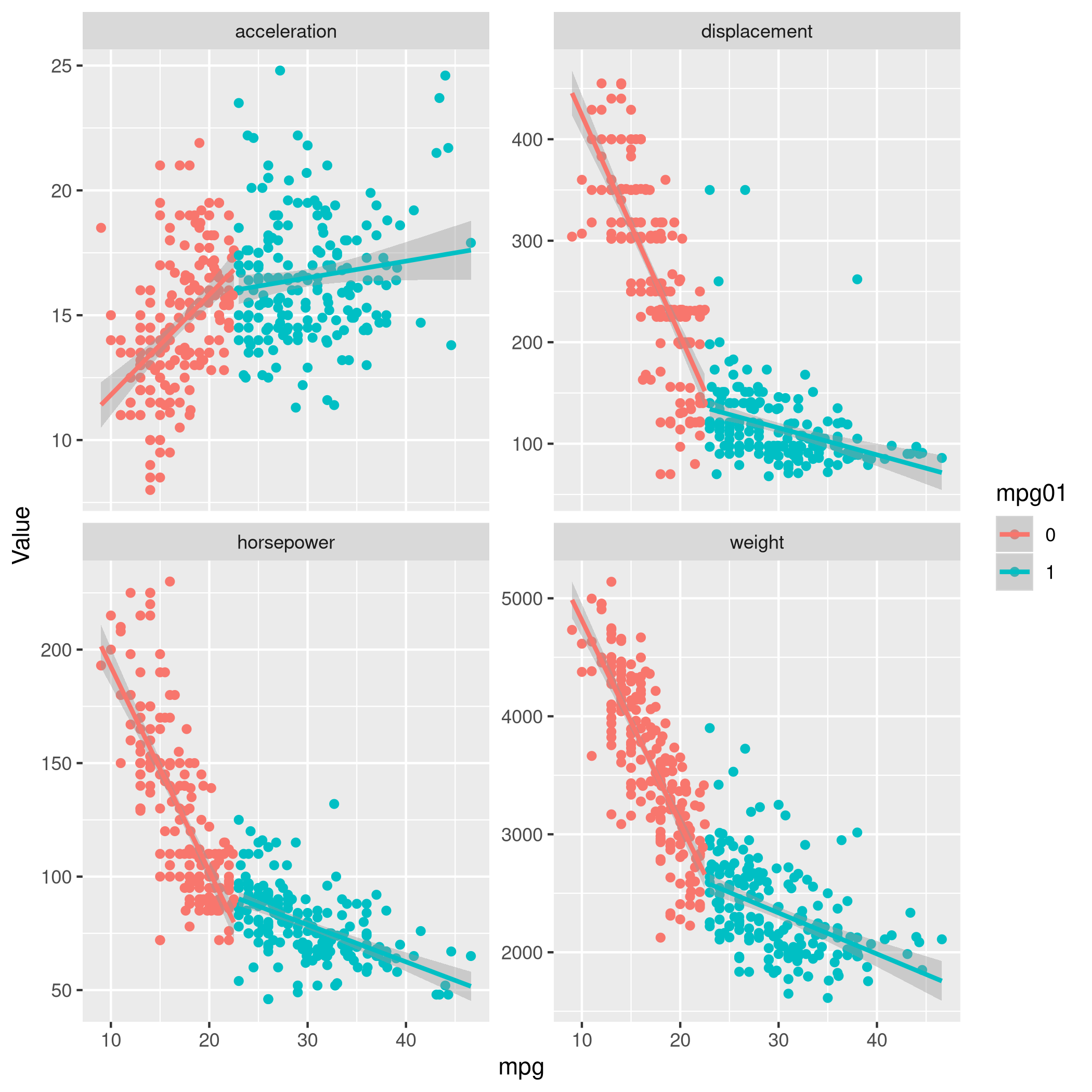
1newDat %>% select(-year,-origin,-cylinders) %>% pivot_longer(-c(mpg01,name,mpg),names_to="Params",values_to="Value") %>% ggplot(aes(x=mpg,y=Value,color=mpg01)) +
2  geom_point() +
3  geom_smooth(method=lm) +
4  facet_wrap(~ Params, scales = "free_y")
c) Train-Test Split
We can split our data
very
easily with caret. It is important to remember that for factors,
random sampling occurs within each class to preserve the overall class
distribution of the data.
1set.seed(1984)
2trainInd <- createDataPartition(newDat$mpg01, # Factor, so class sampling
3                                p=0.7, # 70-30 train-test
4                                list=FALSE, # No lists
5                                times=1) # No bootstrap
6autoTrain<-newDat[trainInd,]
7autoTest<-newDat[-trainInd,]
d) LDA with Significant Variables
Whenever I see significant I think correlation, so let’s take a look at that.
1newDat %>% select(-mpg01,-name) %>% cor
 1#                     mpg  cylinders displacement horsepower     weight
 2# mpg           1.0000000 -0.7776175   -0.8051269 -0.7784268 -0.8322442
 3# cylinders    -0.7776175  1.0000000    0.9508233  0.8429834  0.8975273
 4# displacement -0.8051269  0.9508233    1.0000000  0.8972570  0.9329944
 5# horsepower   -0.7784268  0.8429834    0.8972570  1.0000000  0.8645377
 6# weight       -0.8322442  0.8975273    0.9329944  0.8645377  1.0000000
 7# acceleration  0.4233285 -0.5046834   -0.5438005 -0.6891955 -0.4168392
 8# year          0.5805410 -0.3456474   -0.3698552 -0.4163615 -0.3091199
 9# origin        0.5652088 -0.5689316   -0.6145351 -0.4551715 -0.5850054
10#              acceleration       year     origin
11# mpg             0.4233285  0.5805410  0.5652088
12# cylinders      -0.5046834 -0.3456474 -0.5689316
13# displacement   -0.5438005 -0.3698552 -0.6145351
14# horsepower     -0.6891955 -0.4163615 -0.4551715
15# weight         -0.4168392 -0.3091199 -0.5850054
16# acceleration    1.0000000  0.2903161  0.2127458
17# year            0.2903161  1.0000000  0.1815277
18# origin          0.2127458  0.1815277  1.0000000
1newDat %>% length
1# [1] 10
Now lets quickly see what it looks like with correlated values removed.
1corrCols2=newDat %>% select(-mpg01,-name) %>% cor %>% findCorrelation(cutoff=0.85)
2newRed<-newDat[-c(corrCols2)]
3newRed %>% summary
 1#       mpg            weight      acceleration        year           origin
 2#  Min.   : 9.00   Min.   :1613   Min.   : 8.00   Min.   :70.00   Min.   :1.000
 3#  1st Qu.:17.00   1st Qu.:2225   1st Qu.:13.78   1st Qu.:73.00   1st Qu.:1.000
 4#  Median :22.75   Median :2804   Median :15.50   Median :76.00   Median :1.000
 5#  Mean   :23.45   Mean   :2978   Mean   :15.54   Mean   :75.98   Mean   :1.577
 6#  3rd Qu.:29.00   3rd Qu.:3615   3rd Qu.:17.02   3rd Qu.:79.00   3rd Qu.:2.000
 7#  Max.   :46.60   Max.   :5140   Max.   :24.80   Max.   :82.00   Max.   :3.000
 8#
 9#                  name     mpg01
10#  amc matador       :  5   0:196
11#  ford pinto        :  5   1:196
12#  toyota corolla    :  5
13#  amc gremlin       :  4
14#  amc hornet        :  4
15#  chevrolet chevette:  4
16#  (Other)           :365
Inherent in this discussion is the fact that I consider what is
correlated to mpg to be a good indicator of what will help mpg01 for
obvious reasons.
Now we can just use the columns we found with findCorrelation.
1corrCols2 %>% print
1# [1] 3 4 2
1names(newDat)
1#  [1] "mpg"          "cylinders"    "displacement" "horsepower"   "weight"
2#  [6] "acceleration" "year"         "origin"       "name"         "mpg01"
1autoLDA=train(mpg01~cylinders+displacement+horsepower,data=autoTrain,method="lda")
2valScoreLDA=predict(autoLDA,autoTest)
Now we can check the statistics.
1confusionMatrix(valScoreLDA,autoTest$mpg01)
 1# Confusion Matrix and Statistics
 2#
 3#           Reference
 4# Prediction  0  1
 5#          0 56  2
 6#          1  2 56
 7#
 8#                Accuracy : 0.9655
 9#                  95% CI : (0.9141, 0.9905)
10#     No Information Rate : 0.5
11#     P-Value [Acc > NIR] : <2e-16
12#
13#                   Kappa : 0.931
14#
15#  Mcnemar's Test P-Value : 1
16#
17#             Sensitivity : 0.9655
18#             Specificity : 0.9655
19#          Pos Pred Value : 0.9655
20#          Neg Pred Value : 0.9655
21#              Prevalence : 0.5000
22#          Detection Rate : 0.4828
23#    Detection Prevalence : 0.5000
24#       Balanced Accuracy : 0.9655
25#
26#        'Positive' Class : 0
27#
That is an amazingly accurate model.
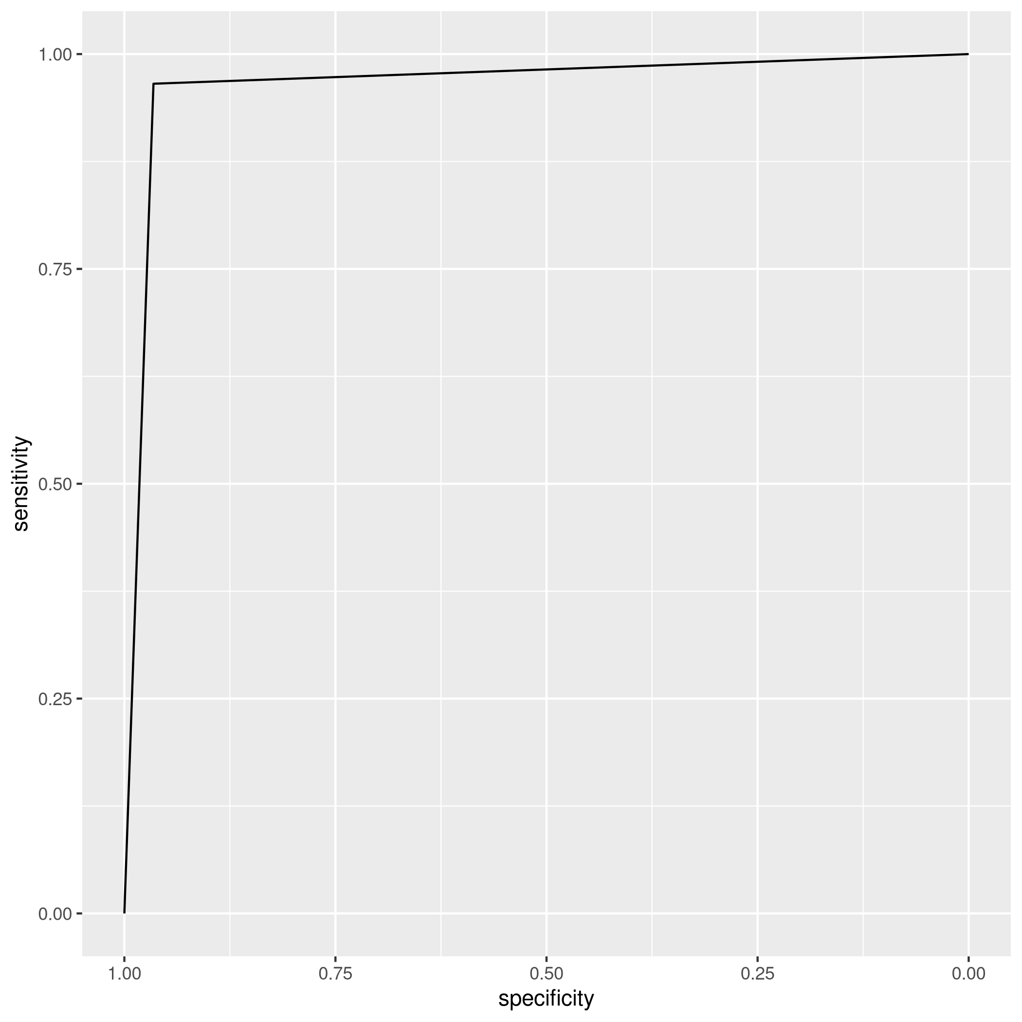
1auto_ldaROC<-roc(predictor=as.numeric(valScoreLDA),response=autoTest$mpg01,levels=levels(autoTest$mpg01))
1# Setting direction: controls < cases
1ggroc(auto_ldaROC)

e) QDA with Significant Variables
Same deal as before.
1autoQDA=train(mpg01~cylinders+displacement+horsepower,data=autoTrain,method="qda")
2valScoreQDA=predict(autoQDA,autoTest)
Now we can check the statistics.
1confusionMatrix(valScoreQDA,autoTest$mpg01)
 1# Confusion Matrix and Statistics
 2#
 3#           Reference
 4# Prediction  0  1
 5#          0 56  2
 6#          1  2 56
 7#
 8#                Accuracy : 0.9655
 9#                  95% CI : (0.9141, 0.9905)
10#     No Information Rate : 0.5
11#     P-Value [Acc > NIR] : <2e-16
12#
13#                   Kappa : 0.931
14#
15#  Mcnemar's Test P-Value : 1
16#
17#             Sensitivity : 0.9655
18#             Specificity : 0.9655
19#          Pos Pred Value : 0.9655
20#          Neg Pred Value : 0.9655
21#              Prevalence : 0.5000
22#          Detection Rate : 0.4828
23#    Detection Prevalence : 0.5000
24#       Balanced Accuracy : 0.9655
25#
26#        'Positive' Class : 0
27#
1auto_qdaROC<-roc(predictor=as.numeric(valScoreQDA),response=autoTest$mpg01,levels=levels(autoTest$mpg01))
1# Setting direction: controls < cases
1ggroc(auto_qdaROC)
OK, this is weird enough to check if it isn’t some sort of artifact.
1autoQDA2=train(mpg01~horsepower, data=autoTrain,method='qda')
2valScoreQDA2=predict(autoQDA2, autoTest)
3confusionMatrix(valScoreQDA2,autoTest$mpg01)
 1# Confusion Matrix and Statistics
 2#
 3#           Reference
 4# Prediction  0  1
 5#          0 42  3
 6#          1 16 55
 7#
 8#                Accuracy : 0.8362
 9#                  95% CI : (0.7561, 0.8984)
10#     No Information Rate : 0.5
11#     P-Value [Acc > NIR] : 4.315e-14
12#
13#                   Kappa : 0.6724
14#
15#  Mcnemar's Test P-Value : 0.005905
16#
17#             Sensitivity : 0.7241
18#             Specificity : 0.9483
19#          Pos Pred Value : 0.9333
20#          Neg Pred Value : 0.7746
21#              Prevalence : 0.5000
22#          Detection Rate : 0.3621
23#    Detection Prevalence : 0.3879
24#       Balanced Accuracy : 0.8362
25#
26#        'Positive' Class : 0
27#
OK, so the model isn’t completely creepily correct all the time. In this
case we should probably think about what is going on. I would think it
is because of the nature of the train-test split we performed. We have
ensured during the sampling of our data that the train and test sets
contain the SAME distribution (assumed). So that’s why our training
result and test results are both incredibly good. They’re essentially
the same thing.
In fact, this is the perfect time to consider a validation set, just to see what the models are really doing. Won’t get into it right now though.
f) Logistic with Significant Variables
1glmAuto.fit=glm(mpg01~cylinders+displacement+horsepower, data=autoTrain, family=binomial)
1glmAuto.probs = predict(glmAuto.fit,autoTest, type = "response")
2glmAuto.pred = rep(1,length(glmAuto.probs))
3glmAuto.pred[glmAuto.probs<0.5]=0
4glmAuto.pred=factor(glmAuto.pred)
5confusionMatrix(glmAuto.pred,autoTest$mpg01)
 1# Confusion Matrix and Statistics
 2#
 3#           Reference
 4# Prediction  0  1
 5#          0 56  4
 6#          1  2 54
 7#
 8#                Accuracy : 0.9483
 9#                  95% CI : (0.8908, 0.9808)
10#     No Information Rate : 0.5
11#     P-Value [Acc > NIR] : <2e-16
12#
13#                   Kappa : 0.8966
14#
15#  Mcnemar's Test P-Value : 0.6831
16#
17#             Sensitivity : 0.9655
18#             Specificity : 0.9310
19#          Pos Pred Value : 0.9333
20#          Neg Pred Value : 0.9643
21#              Prevalence : 0.5000
22#          Detection Rate : 0.4828
23#    Detection Prevalence : 0.5172
24#       Balanced Accuracy : 0.9483
25#
26#        'Positive' Class : 0
27#
g) KNN Modeling
Scale the parameters later.
1knnAuto=train(mpg01~cylinders+displacement+horsepower,data=autoTrain,method="knn")
Plot KNN with the best parameters.
1plot(knnCaret)

Evidently, the accuracy increases with an increase in the number of neighbors considered.
1plot(knnAuto, print.thres = 0.5, type="S")
So we can see that \(5\) neighbors is a good compromise.
Question 4.12 - Pages 172-173
This problem involves writing functions.
(a) Write a function, Power() , that prints out the result of
raising 2 to the 3rd power. In other words, your function should compute
2^3 and print out the results.
Hint: Recall that x^a raises x to the power a. Use the print()
function to output the result.
(b) Create a new function, Power2() , that allows you to pass any
two numbers, x and a , and prints out the value of x^a . You can
do this by beginning your function with the line
1Power2=function(x,a){}
You should be able to call your function by entering, for instance,
1Power2(3,8)
on the command line. This should output the value of \(3^8\), namely, \(6,651\).
(c) Using the Power2() function that you just wrote, compute \(10^3\),
\(8^{17}\), and \(131^3\).
(d) Now create a new function, Power3(), that actually returns the
result x^a as an R object, rather than simply printing it to the
screen. That is, if you store the value x^a in an object called
result within your function, then you can simply return() this
result, using the following line:
1return(result)
The line above should be the last line in your function, before the }
symbol.
(e) Now using the Power3() function, create a plot of \(f(x)=x^2\).
The x-axis should display a range of integers from \(1\) to \(10\), and
the y-axis should display \(x^2\) . Label the axes appropriately, and
use an appropriate title for the figure. Consider displaying either the
x-axis, the y-axis, or both on the log-scale. You can do this by
using log=‘‘x’’, log=‘‘y’’, or log=‘‘xy’’ as arguments to the
plot() function.
(f) Create a function, PlotPower() , that allows you to create a
plot of x against x^a for a fixed a and for a range of values of
x. For instance, if you call
1PlotPower (1:10 ,3)
then a plot should be created with an x-axis taking on values \(1,2,…,10\) and a y-axis taking on values \(1^3,2^3,…,10^3\)
Answer
a) Create a Squaring Function
1Power=function(x){print(2^x)}
2Power(3)
1# [1] 8
b) Generalizing Power to arbitrary numbers
1Power2=function(x,a){print(x^a)}
1Power2(3,8)
1# [1] 6561
c) Random Testing of Power2
1Power2(10,3)
1# [1] 1000
1Power2(8,17)
1# [1] 2.2518e+15
1Power2(131,2)
1# [1] 17161
d) Return a value
1Power3=function(x,a){return(x^a)}
e) Plot something with Power3
Actually now would be a good place to introduce LaTeX labeling.
1#install.packages("latex2exp")
2library(latex2exp)
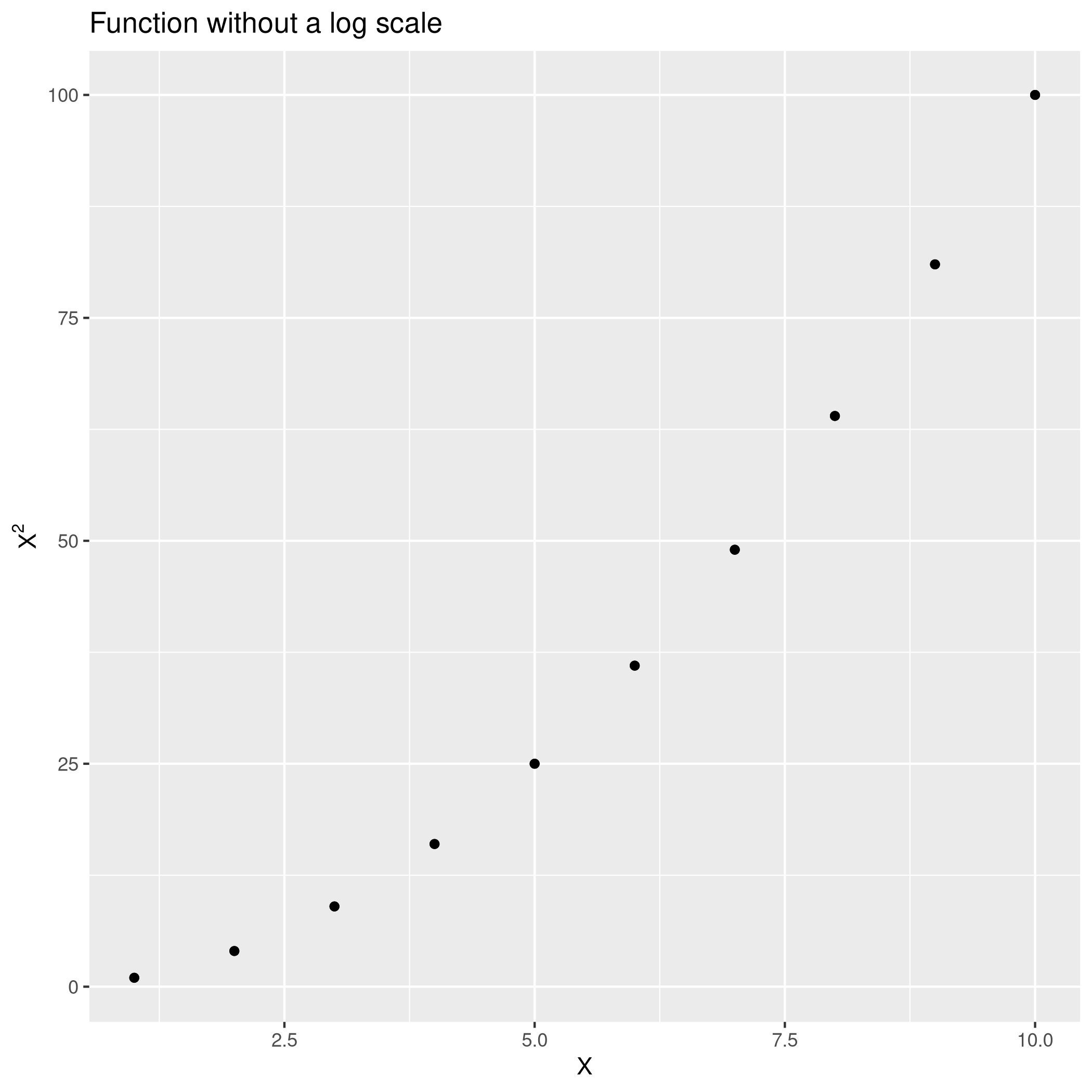
No log scale.
1qplot(x=seq(1,10),y=Power3(seq(1,10),2)) + ggtitle("Function without a log scale") +
2  geom_point() + xlab("X") + ylab(TeX("$X^2$"))
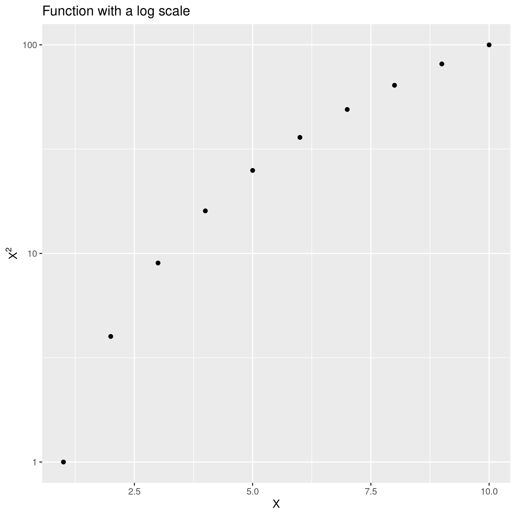
With a log scale.
1qplot(x=seq(1,10),y=Power3(seq(1,10),2)) + ggtitle("Function with a log scale") +
2  geom_point() + xlab("X") + ylab(TeX("$X^2$")) + scale_y_log10()
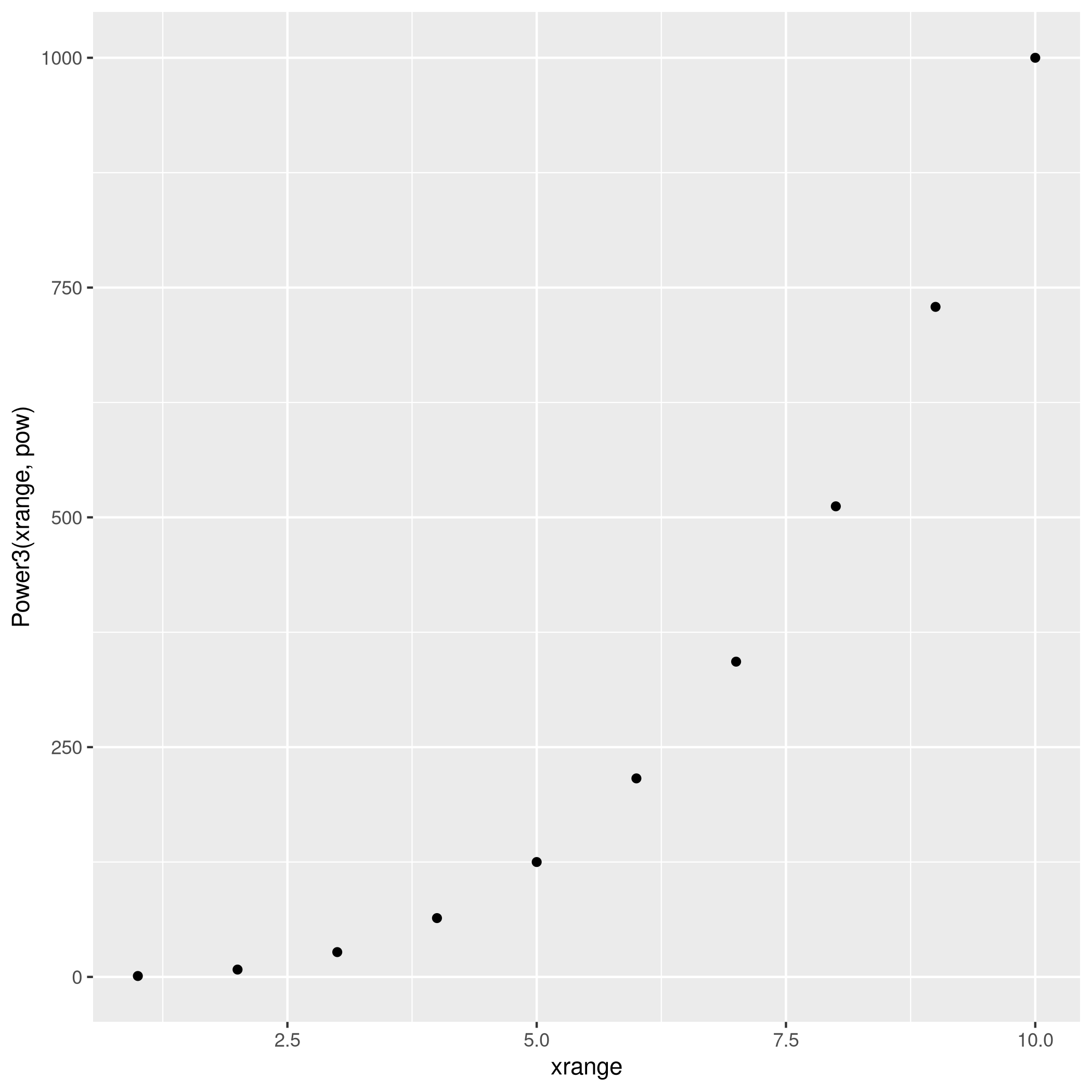
f) PlotPower Function
1PlotPower=function(xrange,pow){return(qplot(x=xrange,y=Power3(xrange,pow)))}
1plotter<-PlotPower(1:10,3)
2plotter
The R Cookbook is quite neat for some simple tasks like this.
Question 4.13 - Pages 173
Using the Boston data set, fit classification models in order to
predict whether a given suburb has a crime rate above or below the
median. Explore logistic regression, LDA, and KNN models using various
subsets of the predictors. Describe your findings.
Answer
OK, to speed this up, I will simply run through all the work done on the
Auto set. Recall that details about this data-set are
also
here.
1boston<-MASS::Boston
- Check unique values
1boston %>% sapply(unique) %>% sapply(length)
1#    crim      zn   indus    chas     nox      rm     age     dis     rad     tax
2#     504      26      76       2      81     446     356     412       9      66
3# ptratio   black   lstat    medv
4#      46     357     455     229
CHAS is of course something which should be a factor, and with RAD
having only \(9\) levels, I’m inclined to make it a factor as well.
1boston<-boston %>% mutate(rad=factor(rad),chas=factor(chas))
- Make a median variable
1boston$highCrime<- ifelse(boston$crim<boston$crim %>% median(),0,1) %>% factor()
- Take a look at the data
Some box-plots:
1boston %>% pivot_longer(-c(rad,chas,highCrime),names_to="Param",values_to="Value") %>% ggplot(aes(x=highCrime,y=Value,fill=chas)) +
2  geom_boxplot()+
3  facet_wrap(~Param,scales="free_y")
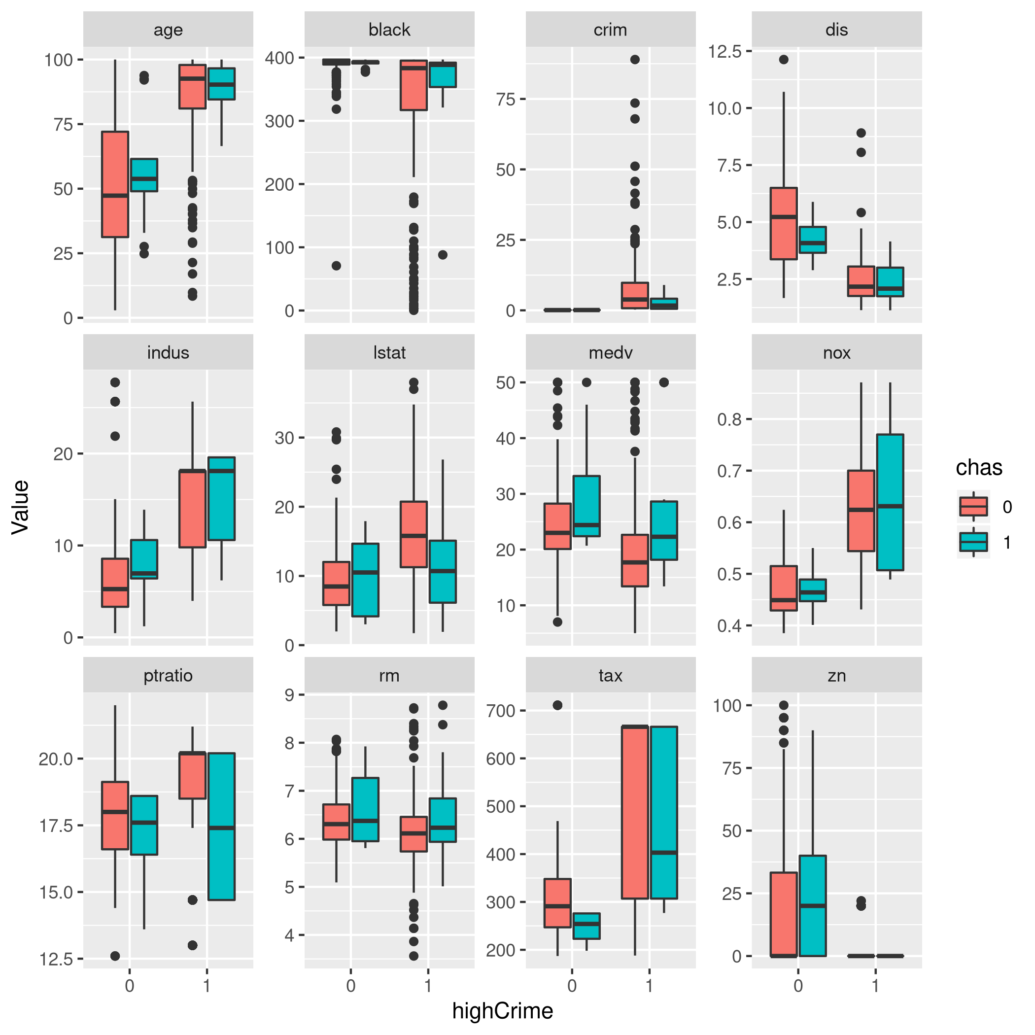
It is surprising, but evidently the CHAS variable is strangely
relevant. 1 implies the tract bounds the river, otherwise 0.
- Correlations
1boston %>% select(-c(rad,chas,highCrime)) %>% cor
 1#               crim         zn      indus        nox         rm        age
 2# crim     1.0000000 -0.2004692  0.4065834  0.4209717 -0.2192467  0.3527343
 3# zn      -0.2004692  1.0000000 -0.5338282 -0.5166037  0.3119906 -0.5695373
 4# indus    0.4065834 -0.5338282  1.0000000  0.7636514 -0.3916759  0.6447785
 5# nox      0.4209717 -0.5166037  0.7636514  1.0000000 -0.3021882  0.7314701
 6# rm      -0.2192467  0.3119906 -0.3916759 -0.3021882  1.0000000 -0.2402649
 7# age      0.3527343 -0.5695373  0.6447785  0.7314701 -0.2402649  1.0000000
 8# dis     -0.3796701  0.6644082 -0.7080270 -0.7692301  0.2052462 -0.7478805
 9# tax      0.5827643 -0.3145633  0.7207602  0.6680232 -0.2920478  0.5064556
10# ptratio  0.2899456 -0.3916785  0.3832476  0.1889327 -0.3555015  0.2615150
11# black   -0.3850639  0.1755203 -0.3569765 -0.3800506  0.1280686 -0.2735340
12# lstat    0.4556215 -0.4129946  0.6037997  0.5908789 -0.6138083  0.6023385
13# medv    -0.3883046  0.3604453 -0.4837252 -0.4273208  0.6953599 -0.3769546
14#                dis        tax    ptratio      black      lstat       medv
15# crim    -0.3796701  0.5827643  0.2899456 -0.3850639  0.4556215 -0.3883046
16# zn       0.6644082 -0.3145633 -0.3916785  0.1755203 -0.4129946  0.3604453
17# indus   -0.7080270  0.7207602  0.3832476 -0.3569765  0.6037997 -0.4837252
18# nox     -0.7692301  0.6680232  0.1889327 -0.3800506  0.5908789 -0.4273208
19# rm       0.2052462 -0.2920478 -0.3555015  0.1280686 -0.6138083  0.6953599
20# age     -0.7478805  0.5064556  0.2615150 -0.2735340  0.6023385 -0.3769546
21# dis      1.0000000 -0.5344316 -0.2324705  0.2915117 -0.4969958  0.2499287
22# tax     -0.5344316  1.0000000  0.4608530 -0.4418080  0.5439934 -0.4685359
23# ptratio -0.2324705  0.4608530  1.0000000 -0.1773833  0.3740443 -0.5077867
24# black    0.2915117 -0.4418080 -0.1773833  1.0000000 -0.3660869  0.3334608
25# lstat   -0.4969958  0.5439934  0.3740443 -0.3660869  1.0000000 -0.7376627
26# medv     0.2499287 -0.4685359 -0.5077867  0.3334608 -0.7376627  1.0000000
Now, unsurprisingly, there’s nothing which is really strongly correlated here for some reason.
- Train test splits
1set.seed(1984)
2trainIndCri <- createDataPartition(boston$highCrime, # Factor, so class sampling
3                                p=0.7, # 70-30 train-test
4                                list=FALSE, # No lists
5                                times=1) # No bootstrap
6bostonTrain<-boston[trainIndCri,]
7bostonTest<-boston[-trainIndCri,]
- Make a bunch of models
1glmBos.fit=glm(highCrime~., data=bostonTrain, family=binomial)
1# Warning: glm.fit: algorithm did not converge
1# Warning: glm.fit: fitted probabilities numerically 0 or 1 occurred
1glmBos.probs = predict(glmBos.fit,bostonTest, type = "response")
2glmBos.pred = rep(1,length(glmBos.probs))
3glmBos.pred[glmBos.probs<0.5]=0
4glmBos.pred=factor(glmBos.pred)
5confusionMatrix(glmBos.pred,bostonTest$highCrime)
 1# Confusion Matrix and Statistics
 2#
 3#           Reference
 4# Prediction  0  1
 5#          0 68  6
 6#          1  7 69
 7#
 8#                Accuracy : 0.9133
 9#                  95% CI : (0.8564, 0.953)
10#     No Information Rate : 0.5
11#     P-Value [Acc > NIR] : <2e-16
12#
13#                   Kappa : 0.8267
14#
15#  Mcnemar's Test P-Value : 1
16#
17#             Sensitivity : 0.9067
18#             Specificity : 0.9200
19#          Pos Pred Value : 0.9189
20#          Neg Pred Value : 0.9079
21#              Prevalence : 0.5000
22#          Detection Rate : 0.4533
23#    Detection Prevalence : 0.4933
24#       Balanced Accuracy : 0.9133
25#
26#        'Positive' Class : 0
27#
1bostonLDA=train(highCrime~.,data=bostonTrain,method='lda')
2bostonQDA=train(highCrime~tax+crim,data=bostonTrain,method='qda')
3bostonKNN=train(highCrime~.,data=bostonTrain,preProcess = c("center","scale"),method='knn')
1bLDAp=predict(bostonLDA,bostonTest)
2bQDAp=predict(bostonQDA,bostonTest)
3bKNNp=predict(bostonKNN,bostonTest)
1confusionMatrix(bLDAp,bostonTest$highCrime)
 1# Confusion Matrix and Statistics
 2#
 3#           Reference
 4# Prediction  0  1
 5#          0 72  6
 6#          1  3 69
 7#
 8#                Accuracy : 0.94
 9#                  95% CI : (0.8892, 0.9722)
10#     No Information Rate : 0.5
11#     P-Value [Acc > NIR] : <2e-16
12#
13#                   Kappa : 0.88
14#
15#  Mcnemar's Test P-Value : 0.505
16#
17#             Sensitivity : 0.9600
18#             Specificity : 0.9200
19#          Pos Pred Value : 0.9231
20#          Neg Pred Value : 0.9583
21#              Prevalence : 0.5000
22#          Detection Rate : 0.4800
23#    Detection Prevalence : 0.5200
24#       Balanced Accuracy : 0.9400
25#
26#        'Positive' Class : 0
27#
1confusionMatrix(bQDAp,bostonTest$highCrime)
 1# Confusion Matrix and Statistics
 2#
 3#           Reference
 4# Prediction  0  1
 5#          0 73  5
 6#          1  2 70
 7#
 8#                Accuracy : 0.9533
 9#                  95% CI : (0.9062, 0.981)
10#     No Information Rate : 0.5
11#     P-Value [Acc > NIR] : <2e-16
12#
13#                   Kappa : 0.9067
14#
15#  Mcnemar's Test P-Value : 0.4497
16#
17#             Sensitivity : 0.9733
18#             Specificity : 0.9333
19#          Pos Pred Value : 0.9359
20#          Neg Pred Value : 0.9722
21#              Prevalence : 0.5000
22#          Detection Rate : 0.4867
23#    Detection Prevalence : 0.5200
24#       Balanced Accuracy : 0.9533
25#
26#        'Positive' Class : 0
27#
1confusionMatrix(bKNNp,bostonTest$highCrime)
 1# Confusion Matrix and Statistics
 2#
 3#           Reference
 4# Prediction  0  1
 5#          0 74  6
 6#          1  1 69
 7#
 8#                Accuracy : 0.9533
 9#                  95% CI : (0.9062, 0.981)
10#     No Information Rate : 0.5
11#     P-Value [Acc > NIR] : <2e-16
12#
13#                   Kappa : 0.9067
14#
15#  Mcnemar's Test P-Value : 0.1306
16#
17#             Sensitivity : 0.9867
18#             Specificity : 0.9200
19#          Pos Pred Value : 0.9250
20#          Neg Pred Value : 0.9857
21#              Prevalence : 0.5000
22#          Detection Rate : 0.4933
23#    Detection Prevalence : 0.5333
24#       Balanced Accuracy : 0.9533
25#
26#        'Positive' Class : 0
27#
Clearly in this particular case, an LDA model seems to be working out the best for this data when trained on all the parameters, though Logistic Regression is doing quite well too.
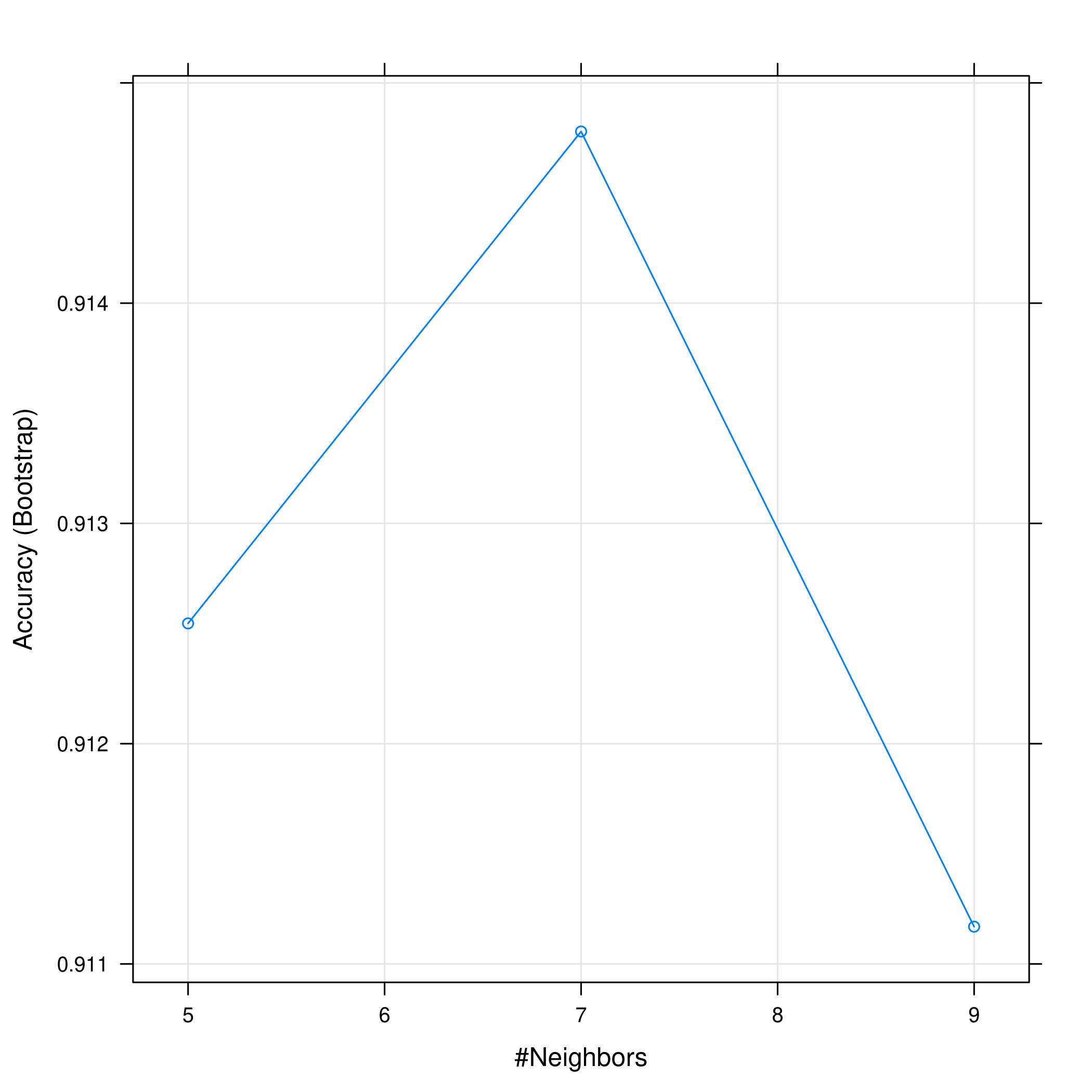
- Notes on KNN
1plot(bostonKNN)
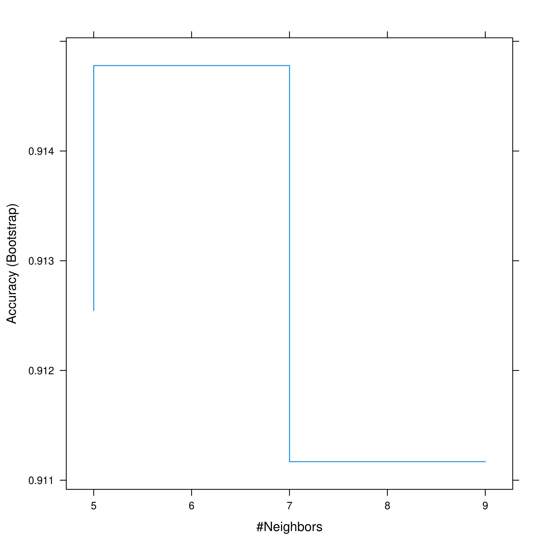
1plot(bostonKNN, print.thres = 0.5, type="S")
- Comparison
Finally, we will quickly plot some indicative measures.
1knnBosROC<-roc(predictor=as.numeric(bKNNp),response=bostonTest$highCrime)
1# Setting levels: control = 0, case = 1
1# Setting direction: controls < cases
1logiBosROC<-roc(predictor=as.numeric(glmBos.probs),response=bostonTest$highCrime)
1# Setting levels: control = 0, case = 1
2# Setting direction: controls < cases
1ldaBosROC<-roc(predictor=as.numeric(bLDAp),response=bostonTest$highCrime)
1# Setting levels: control = 0, case = 1
2# Setting direction: controls < cases
1qdaBosROC<-roc(predictor=as.numeric(bQDAp),response=bostonTest$highCrime)
1# Setting levels: control = 0, case = 1
2# Setting direction: controls < cases
1ggroc(list(KNN=knnBosROC,Logistic=logiBosROC,LDA=ldaBosROC,QDA=qdaBosROC))
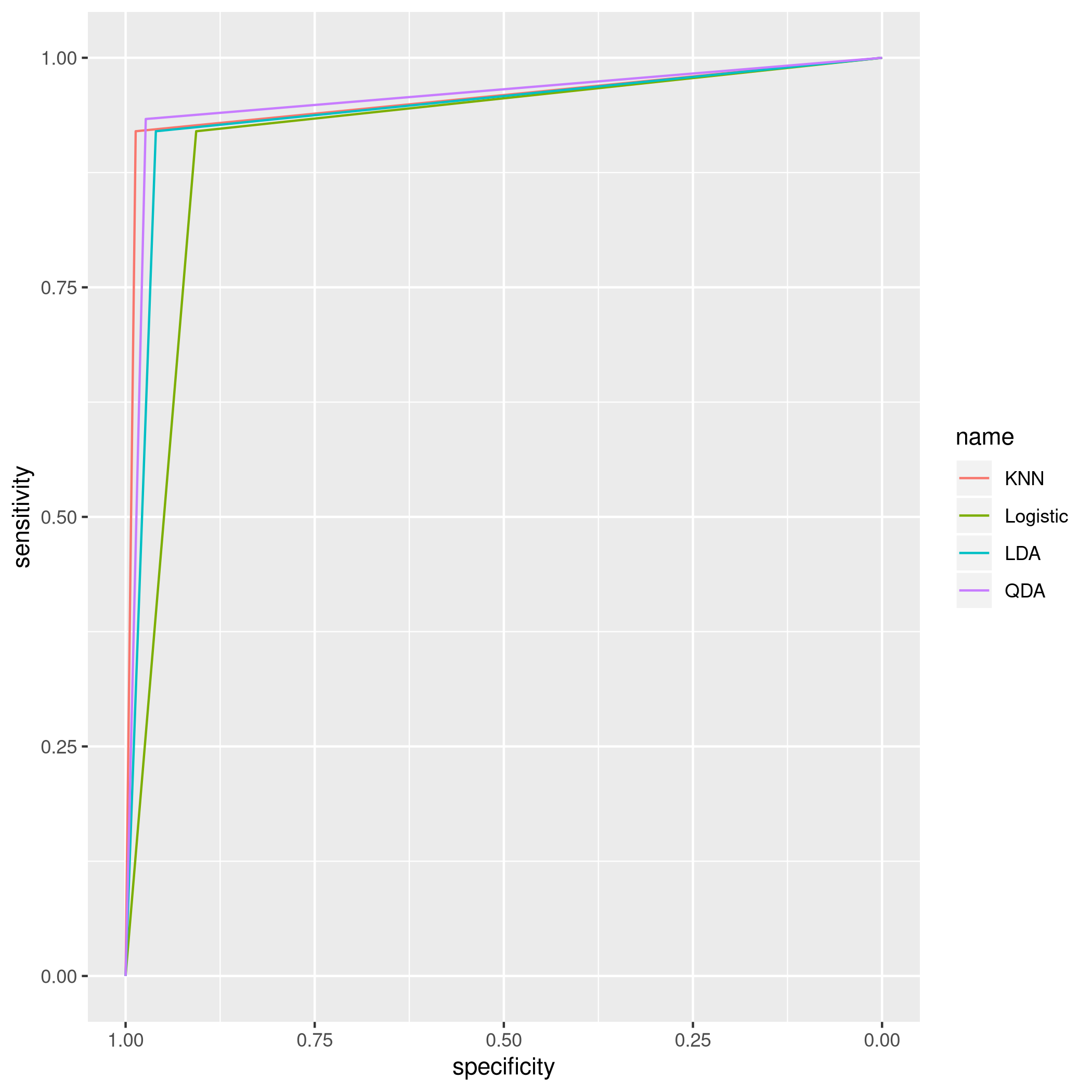
Figure 14: plot of chunk unnamed-chunk-87
OK, one of the reasons why these models do so well is because they are
all assuming an equal distribution of train and test classes, and they
use crim itself as a predictor. This is no doubt a strong reason why
these models uniformly perform so well. I’d say 5 is the best option.
![]()