
25 minutes
Written: 2020-02-18 22:00 +0000
ISLR :: Resampling Methods
Chapter V - Resampling Methods
All the questions are as per the ISL seventh printing of the First edition1.
Common
Instead of using the standard functions, we will leverage the mlr3
package2.
1#install.packages("mlr3","data.table","mlr3viz","mlr3learners")
Actually for R version 3.6.2, the steps to get it working were a bit
more involved.
1install.packages("remotes","data.table",
2                 "GGally","precerec") # For plots
1library(remotes)
2remotes::install_github("mlr-org/mlr3")
3remotes::install_github("mlr-org/mlr3viz")
4remotes::install_github("mlr-org/mlr3learners")
Load ISLR and other libraries.
1libsUsed<-c("dplyr","ggplot2","tidyverse",
2            "ISLR","caret","MASS",
3            "pROC","mlr3","data.table",
4            "mlr3viz","mlr3learners")
5invisible(lapply(libsUsed, library, character.only = TRUE))
Question 5.5 - Page 198
In Chapter 4, we used logistic regression to predict the probability of
default using income and balance on the Default data set. We
will now estimate the test error of this logistic regression model using
the validation set approach. Do not forget to set a random seed before
beginning your analysis.
(a) Fit a logistic regression model that uses income and balance to
predict default.
(b) Using the validation set approach, estimate the test error of this model. In order to do this, you must perform the following steps:
Split the sample set into a training set and a validation set.
Fit a multiple logistic regression model using only the training observations.
Obtain a prediction of default status for each individual in the validation set by computing the posterior probability of default for that individual, and classifying the individual to the
defaultcategory if the posterior probability is greater than \(0.5\).Compute the validation set error, which is the fraction of the observations in the validation set that are misclassified.
(c) Repeat the process in (b) three times, using three different splits of the observations into a training set and a validation set. Comment on the results obtained.
(d) Now consider a logistic regression model that predicts the prob-
ability of default using income , balance , and a dummy variable
for student. Estimate the test error for this model using the
validation set approach. Comment on whether or not including a dummy
variable for student leads to a reduction in the test error rate.
Answer
We will need our data.
1defDat<-ISLR::Default
- Very quick peek
1defDat %>% summary
1##  default    student       balance           income
2##  No :9667   No :7056   Min.   :   0.0   Min.   :  772
3##  Yes: 333   Yes:2944   1st Qu.: 481.7   1st Qu.:21340
4##                        Median : 823.6   Median :34553
5##                        Mean   : 835.4   Mean   :33517
6##                        3rd Qu.:1166.3   3rd Qu.:43808
7##                        Max.   :2654.3   Max.   :73554
1defDat %>% str
1## 'data.frame':    10000 obs. of  4 variables:
2##  $ default: Factor w/ 2 levels "No","Yes": 1 1 1 1 1 1 1 1 1 1 ...
3##  $ student: Factor w/ 2 levels "No","Yes": 1 2 1 1 1 2 1 2 1 1 ...
4##  $ balance: num  730 817 1074 529 786 ...
5##  $ income : num  44362 12106 31767 35704 38463 ...
a) Logistic Model with mlr3
Following the new approach which leverages R6 features leads us to define a classification task first. As far as I can tell, the data needs to be filtered to contain only the things we need to predict with, in this case we are required to use only income and balance so we will do so.
1set.seed(1984)
2redDat<-defDat %>% subset(select=c(income,balance,default))
3tskLogiFull=TaskClassif$new(id="credit",backend=redDat,target="default")
4print(tskLogiFull)
1## <TaskClassif:credit> (10000 x 3)
2## * Target: default
3## * Properties: twoclass
4## * Features (2):
5##   - dbl (2): balance, income
This can be visualized neatly as well.
1autoplot(tskLogiFull)
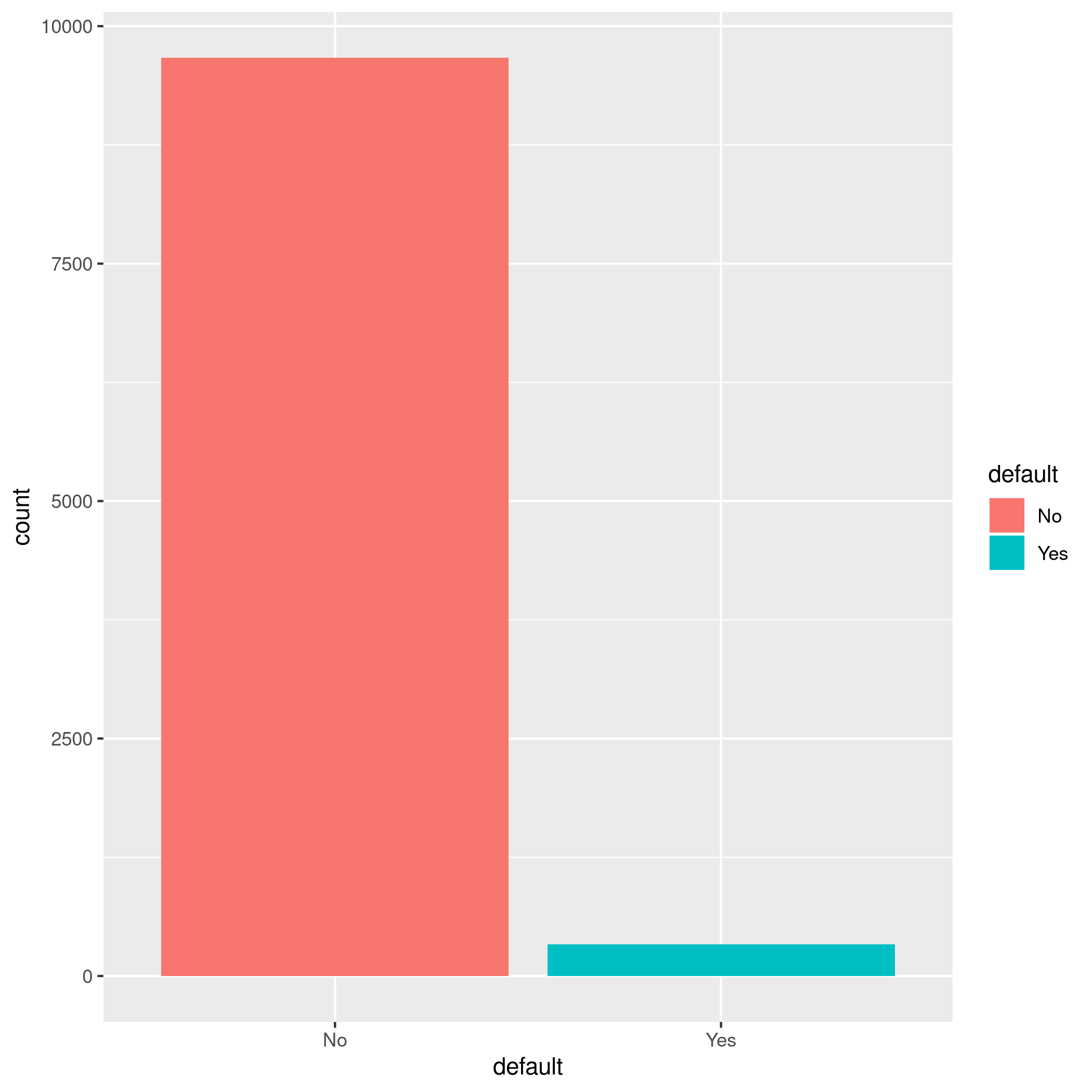
Figure 1: MLR3 Visualizations
We have a pretty imbalanced data-set.
1autoplot(tskLogiFull,type="pairs")
1## Registered S3 method overwritten by 'GGally':
2##   method from
3##   +.gg   ggplot2
1## `stat_bin()` using `bins = 30`. Pick better value with `binwidth`.
2## `stat_bin()` using `bins = 30`. Pick better value with `binwidth`.
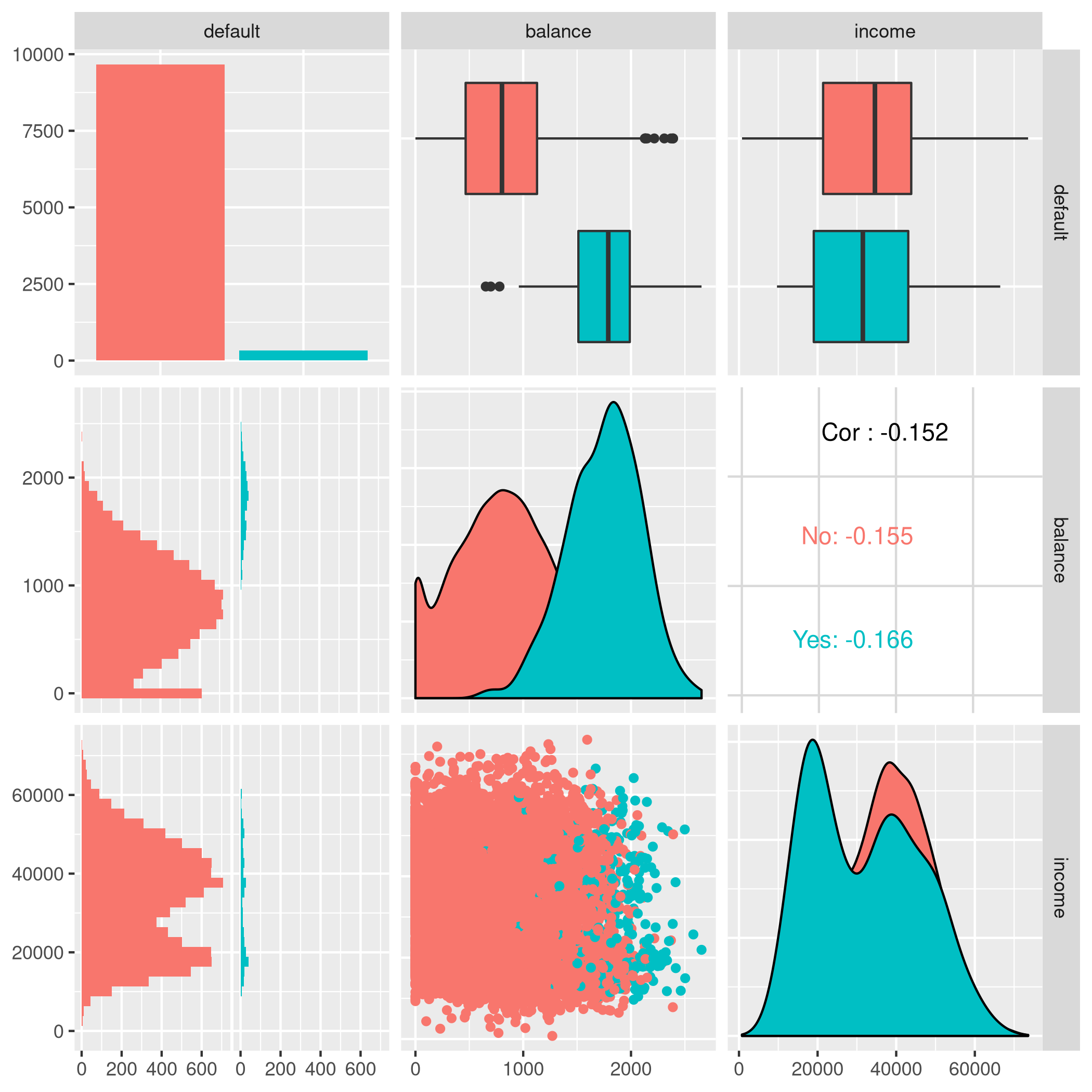
Figure 2: Paired mlr3 data
We can use any of the learners implemented, so it is a good idea to take a quick peek at them all.
1as.data.table(mlr_learners)
 1##                     key                                    feature_types
 2##  1:       classif.debug logical,integer,numeric,character,factor,ordered
 3##  2: classif.featureless logical,integer,numeric,character,factor,ordered
 4##  3:      classif.glmnet                          logical,integer,numeric
 5##  4:        classif.kknn           logical,integer,numeric,factor,ordered
 6##  5:         classif.lda           logical,integer,numeric,factor,ordered
 7##  6:     classif.log_reg logical,integer,numeric,character,factor,ordered
 8##  7: classif.naive_bayes                   logical,integer,numeric,factor
 9##  8:         classif.qda           logical,integer,numeric,factor,ordered
10##  9:      classif.ranger logical,integer,numeric,character,factor,ordered
11## 10:       classif.rpart           logical,integer,numeric,factor,ordered
12## 11:         classif.svm                          logical,integer,numeric
13## 12:     classif.xgboost                          logical,integer,numeric
14## 13:    regr.featureless logical,integer,numeric,character,factor,ordered
15## 14:         regr.glmnet                          logical,integer,numeric
16## 15:           regr.kknn           logical,integer,numeric,factor,ordered
17## 16:             regr.km                          logical,integer,numeric
18## 17:             regr.lm                   logical,integer,numeric,factor
19## 18:         regr.ranger logical,integer,numeric,character,factor,ordered
20## 19:          regr.rpart           logical,integer,numeric,factor,ordered
21## 20:            regr.svm                          logical,integer,numeric
22## 21:        regr.xgboost                          logical,integer,numeric
23##                     key                                    feature_types
24##        packages
25##  1:
26##  2:
27##  3:      glmnet
28##  4:        kknn
29##  5:        MASS
30##  6:       stats
31##  7:       e1071
32##  8:        MASS
33##  9:      ranger
34## 10:       rpart
35## 11:       e1071
36## 12:     xgboost
37## 13:       stats
38## 14:      glmnet
39## 15:        kknn
40## 16: DiceKriging
41## 17:       stats
42## 18:      ranger
43## 19:       rpart
44## 20:       e1071
45## 21:     xgboost
46##        packages
47##                                                            properties
48##  1:                                      missings,multiclass,twoclass
49##  2:         importance,missings,multiclass,selected_features,twoclass
50##  3:                                       multiclass,twoclass,weights
51##  4:                                               multiclass,twoclass
52##  5:                                       multiclass,twoclass,weights
53##  6:                                                  twoclass,weights
54##  7:                                               multiclass,twoclass
55##  8:                                       multiclass,twoclass,weights
56##  9:                  importance,multiclass,oob_error,twoclass,weights
57## 10: importance,missings,multiclass,selected_features,twoclass,weights
58## 11:                                               multiclass,twoclass
59## 12:                   importance,missings,multiclass,twoclass,weights
60## 13:                             importance,missings,selected_features
61## 14:                                                           weights
62## 15:
63## 16:
64## 17:                                                           weights
65## 18:                                      importance,oob_error,weights
66## 19:                     importance,missings,selected_features,weights
67## 20:
68## 21:                                       importance,missings,weights
69##                                                            properties
70##     predict_types
71##  1: response,prob
72##  2: response,prob
73##  3: response,prob
74##  4: response,prob
75##  5: response,prob
76##  6: response,prob
77##  7: response,prob
78##  8: response,prob
79##  9: response,prob
80## 10: response,prob
81## 11: response,prob
82## 12: response,prob
83## 13:   response,se
84## 14:      response
85## 15:      response
86## 16:   response,se
87## 17:   response,se
88## 18:   response,se
89## 19:      response
90## 20:      response
91## 21:      response
92##     predict_types
We can now pick the logistic one.
Note that this essentially
proxies our requests down to the stats package.
1learner = mlr_learners$get("classif.log_reg")
Now we can final solve the question, which is to simply use the model on all our data and return the accuracy metrics.
1trainFullCred=learner$train(tskLogiFull)
2print(learner$predict(tskLogiFull)$confusion)
1##         truth
2## response   No  Yes
3##      No  9629  225
4##      Yes   38  108
1measure = msr("classif.acc")
2print(learner$predict(tskLogiFull)$score(measure))
1## classif.acc
2##      0.9737
Note that this style of working with objects does not really utilize the
familiar %>% interface.
The caret package still has neater default metrics so we will use that
as well.
1confusionMatrix(learner$predict(tskLogiFull)$response,defDat$default)
 1## Confusion Matrix and Statistics
 2##
 3##           Reference
 4## Prediction   No  Yes
 5##        No  9629  225
 6##        Yes   38  108
 7##
 8##                Accuracy : 0.9737
 9##                  95% CI : (0.9704, 0.9767)
10##     No Information Rate : 0.9667
11##     P-Value [Acc > NIR] : 3.067e-05
12##
13##                   Kappa : 0.4396
14##
15##  Mcnemar's Test P-Value : < 2.2e-16
16##
17##             Sensitivity : 0.9961
18##             Specificity : 0.3243
19##          Pos Pred Value : 0.9772
20##          Neg Pred Value : 0.7397
21##              Prevalence : 0.9667
22##          Detection Rate : 0.9629
23##    Detection Prevalence : 0.9854
24##       Balanced Accuracy : 0.6602
25##
26##        'Positive' Class : No
27##
1autoplot(learner$predict(tskLogiFull))

Figure 3: Autoplot results
We can get some other plots as well, but we need our probabilities to be returned.
1# For ROC curves
2lrnprob = lrn("classif.log_reg",predict_type="prob")
3lrnprob$train(tskLogiFull)
4autoplot(lrnprob$predict(tskLogiFull),type="roc")
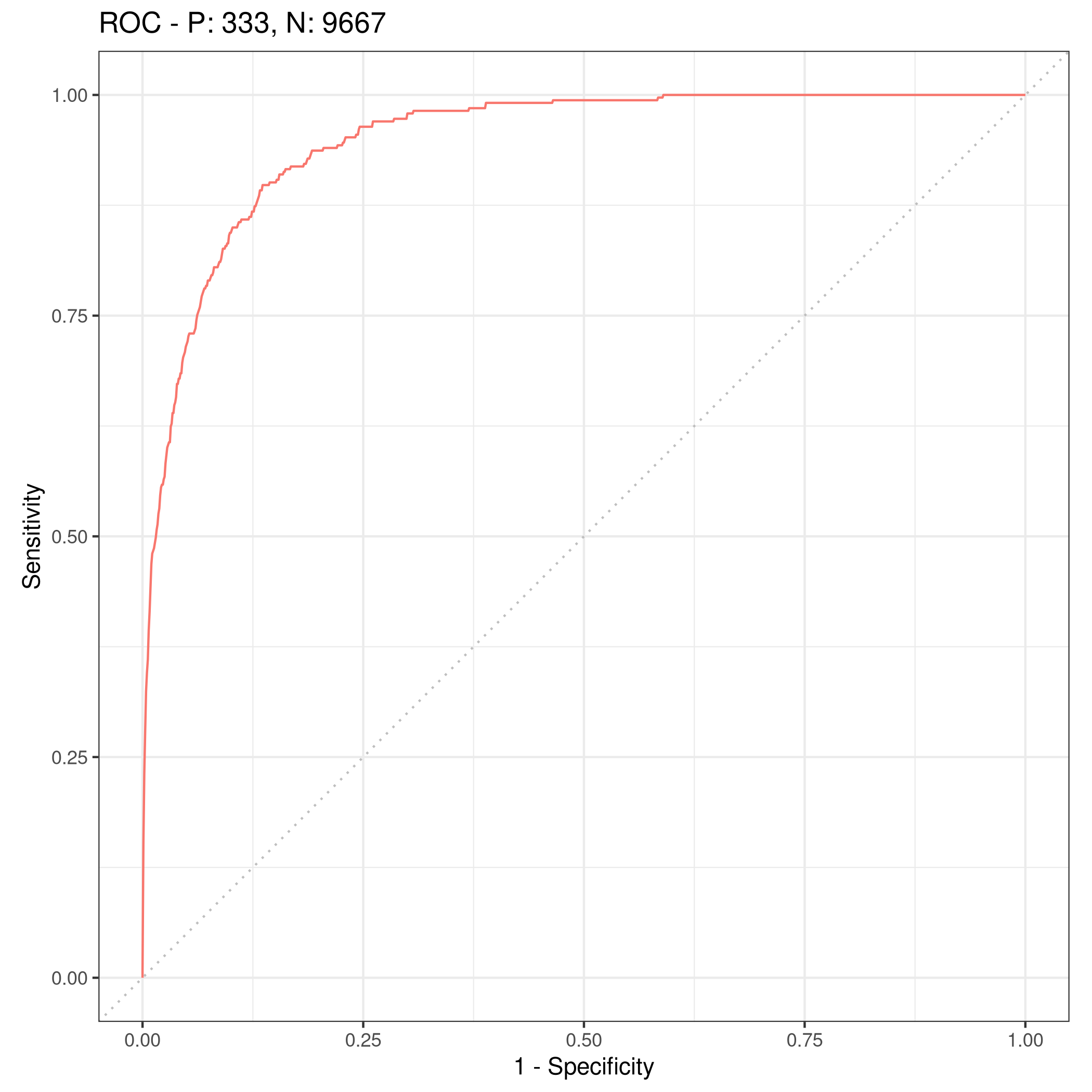
Figure 4: ROC curve
b) Validation Sets with mlr3
Though the question seems to require a manual validation set generation and thresholding, we can simply use the defaults.
1train_set = sample(tskLogiFull$nrow, 0.8 * tskLogiFull$nrow)
2test_set = setdiff(seq_len(tskLogiFull$nrow), train_set)
3learner$train(tskLogiFull,row_ids=train_set)
4confusionMatrix(learner$predict(tskLogiFull, row_ids=test_set)$response,defDat[-train_set,]$default)
 1## Confusion Matrix and Statistics
 2##
 3##           Reference
 4## Prediction   No  Yes
 5##        No  1921   47
 6##        Yes    9   23
 7##
 8##                Accuracy : 0.972
 9##                  95% CI : (0.9638, 0.9788)
10##     No Information Rate : 0.965
11##     P-Value [Acc > NIR] : 0.04663
12##
13##                   Kappa : 0.4387
14##
15##  Mcnemar's Test P-Value : 7.641e-07
16##
17##             Sensitivity : 0.9953
18##             Specificity : 0.3286
19##          Pos Pred Value : 0.9761
20##          Neg Pred Value : 0.7188
21##              Prevalence : 0.9650
22##          Detection Rate : 0.9605
23##    Detection Prevalence : 0.9840
24##       Balanced Accuracy : 0.6620
25##
26##        'Positive' Class : No
27##
For a reasonable comparison, we will demonstrate a standard approach as
well. In this instance we will not use caret to ensure that our class
distribution in the train and test sets are not sampled to remain the
same.
1trainNoCaret<-sample(nrow(defDat), size = floor(.8*nrow(defDat)), replace = F)
2glm.fit=glm(default~income+balance,data=defDat,family=binomial,subset=trainNoCaret)
3glm.probs<-predict(glm.fit,defDat[-trainNoCaret,],type="response")
4glm.preds<-ifelse(glm.probs < 0.5, "No", "Yes")
5confusionMatrix(glm.preds %>% factor,defDat[-trainNoCaret,]$default)
 1## Confusion Matrix and Statistics
 2##
 3##           Reference
 4## Prediction   No  Yes
 5##        No  1930   46
 6##        Yes    6   18
 7##
 8##                Accuracy : 0.974
 9##                  95% CI : (0.966, 0.9805)
10##     No Information Rate : 0.968
11##     P-Value [Acc > NIR] : 0.06859
12##
13##                   Kappa : 0.3986
14##
15##  Mcnemar's Test P-Value : 6.362e-08
16##
17##             Sensitivity : 0.9969
18##             Specificity : 0.2812
19##          Pos Pred Value : 0.9767
20##          Neg Pred Value : 0.7500
21##              Prevalence : 0.9680
22##          Detection Rate : 0.9650
23##    Detection Prevalence : 0.9880
24##       Balanced Accuracy : 0.6391
25##
26##        'Positive' Class : No
27##
Since the two approaches use different samples there is a little variation, but we can see that the accuracy is essentially the same.
c) 3-fold cross validation
As per the question, we can repeat the block above three times, or
extract it into a function which takes a seed value and run that three
times. Either way, here we will present the mlr3 approach to cross
validation and resampling.
1rr = resample(tskLogiFull, lrnprob, rsmp("cv", folds = 3))
1## INFO  [22:12:30.025] Applying learner 'classif.log_reg' on task 'credit' (iter 1/3)
2## INFO  [22:12:30.212] Applying learner 'classif.log_reg' on task 'credit' (iter 2/3)
3## INFO  [22:12:30.360] Applying learner 'classif.log_reg' on task 'credit' (iter 3/3)
1autoplot(rr,type="roc")
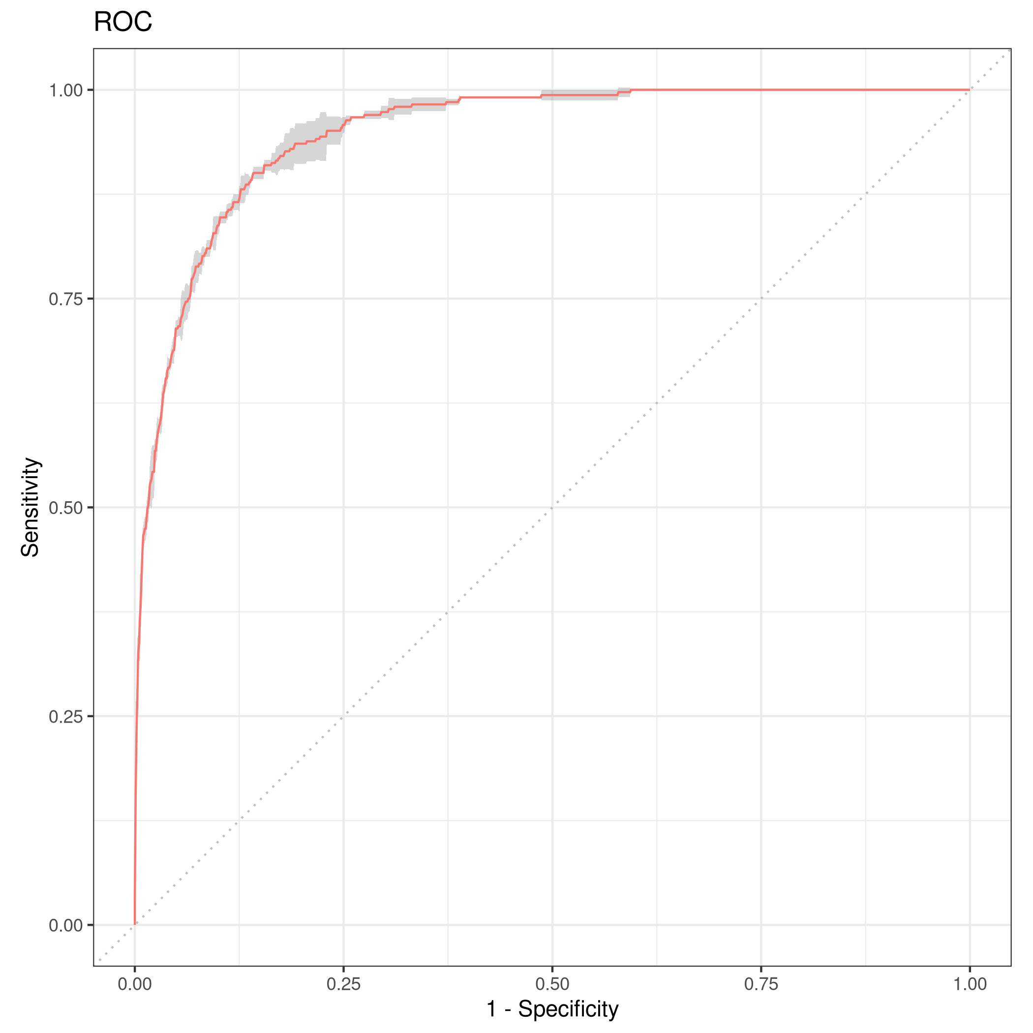
Figure 5: Resampled ROC curve
We might want the average as well.
1rr$aggregate(msr("classif.ce")) %>% print
1## classif.ce
2## 0.02630035
Adding Student as a dummy variable
We will stick to the mlr3 approach because it is faster.
1redDat2<-defDat %>% mutate(student=as.numeric(defDat$student))
2tskLogi2=TaskClassif$new(id="credit",backend=redDat2,target="default")
3print(tskLogi2)
1## <TaskClassif:credit> (10000 x 4)
2## * Target: default
3## * Properties: twoclass
4## * Features (3):
5##   - dbl (3): balance, income, student
1autoplot(tskLogi2,type="pairs")
1## `stat_bin()` using `bins = 30`. Pick better value with `binwidth`.
2## `stat_bin()` using `bins = 30`. Pick better value with `binwidth`.
3## `stat_bin()` using `bins = 30`. Pick better value with `binwidth`.
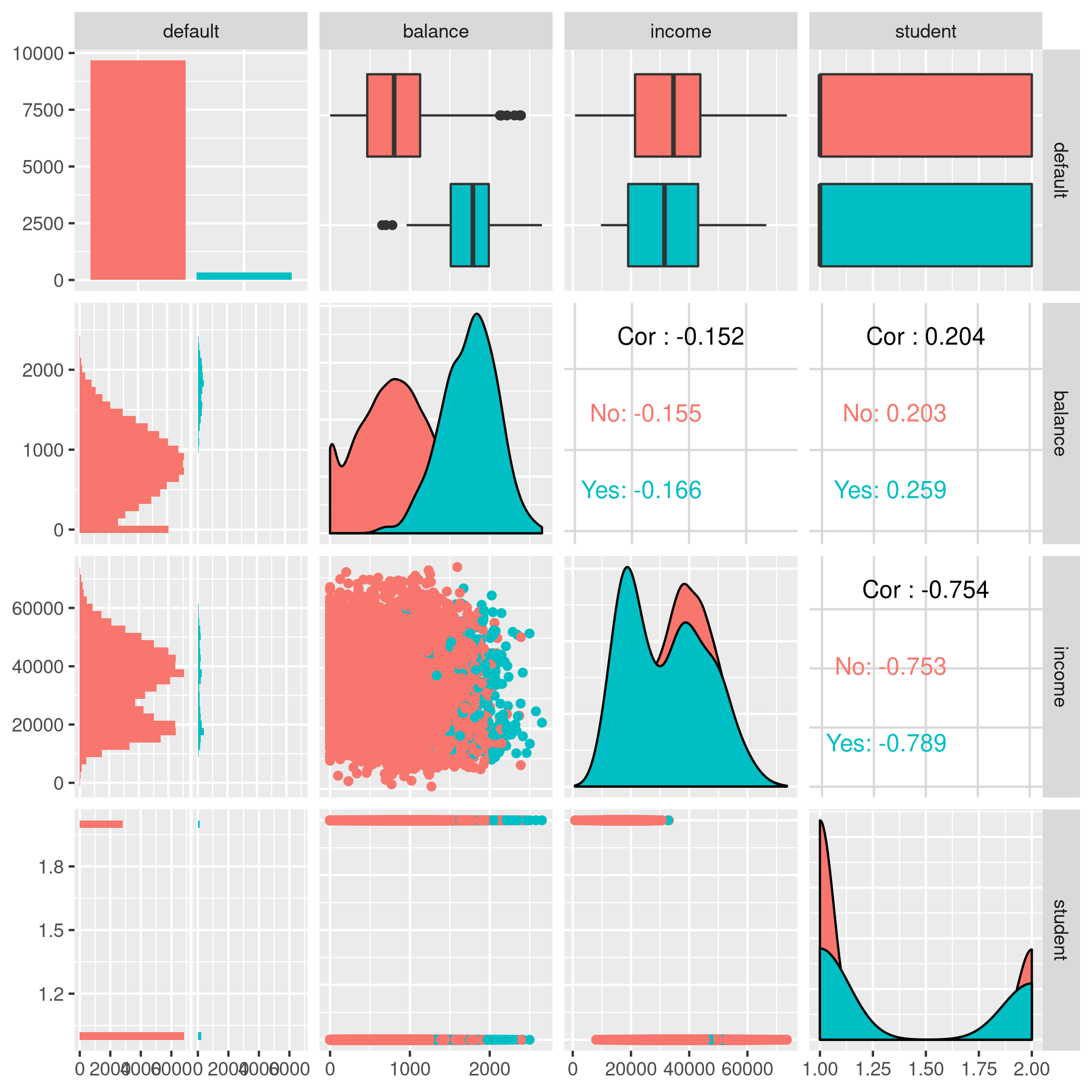
Figure 6: Logistic regression pairs data
This gives us a visual indicator and premonition that we might not be getting incredible results with our new variable in the mix, but we should still work it through.
1confusionMatrix(lrnprob$predict(tskLogi2)$response,defDat$default)
 1## Confusion Matrix and Statistics
 2##
 3##           Reference
 4## Prediction   No  Yes
 5##        No  9629  225
 6##        Yes   38  108
 7##
 8##                Accuracy : 0.9737
 9##                  95% CI : (0.9704, 0.9767)
10##     No Information Rate : 0.9667
11##     P-Value [Acc > NIR] : 3.067e-05
12##
13##                   Kappa : 0.4396
14##
15##  Mcnemar's Test P-Value : < 2.2e-16
16##
17##             Sensitivity : 0.9961
18##             Specificity : 0.3243
19##          Pos Pred Value : 0.9772
20##          Neg Pred Value : 0.7397
21##              Prevalence : 0.9667
22##          Detection Rate : 0.9629
23##    Detection Prevalence : 0.9854
24##       Balanced Accuracy : 0.6602
25##
26##        'Positive' Class : No
27##
1autoplot(lrnprob$predict(tskLogi2))
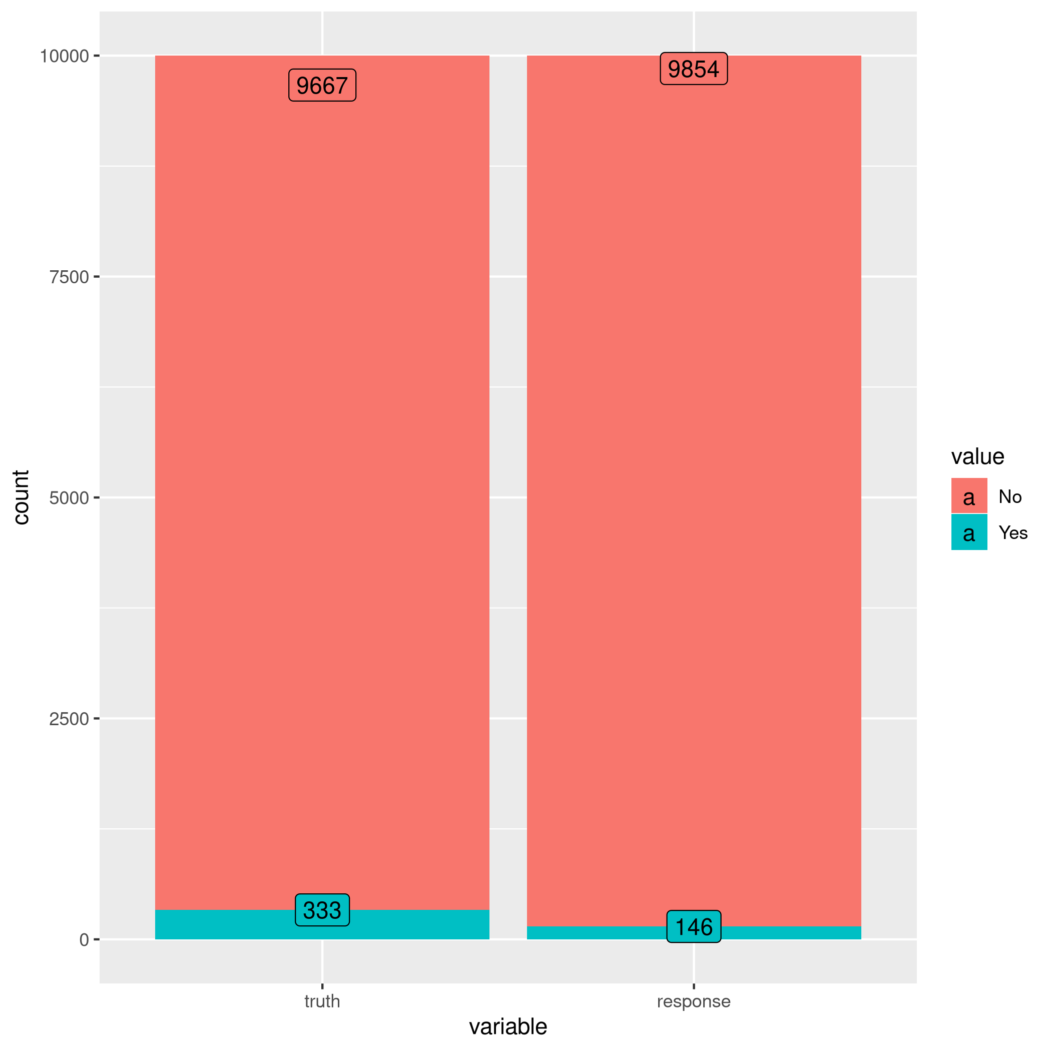
Figure 7: Autoplot figure
1lrnprob$train(tskLogi2)
2autoplot(lrnprob$predict(tskLogi2),type="roc")

Figure 8: ROC plot
Although we have slightly better accuracy with the new variable, it needs to be compared to determine if it is worth further investigation.
With a three-fold validation approach,
1library("gridExtra")
1##
2## Attaching package: 'gridExtra'
1## The following object is masked from 'package:dplyr':
2##
3##     combine
1rr2 = resample(tskLogi2, lrnprob, rsmp("cv", folds = 3))
1## INFO  [22:12:39.670] Applying learner 'classif.log_reg' on task 'credit' (iter 1/3)
2## INFO  [22:12:39.731] Applying learner 'classif.log_reg' on task 'credit' (iter 2/3)
3## INFO  [22:12:39.780] Applying learner 'classif.log_reg' on task 'credit' (iter 3/3)
1wS<-autoplot(rr2)
2nS<-autoplot(rr)
3grid.arrange(wS,nS,ncol=2,bottom="With student (left) and without (right)")
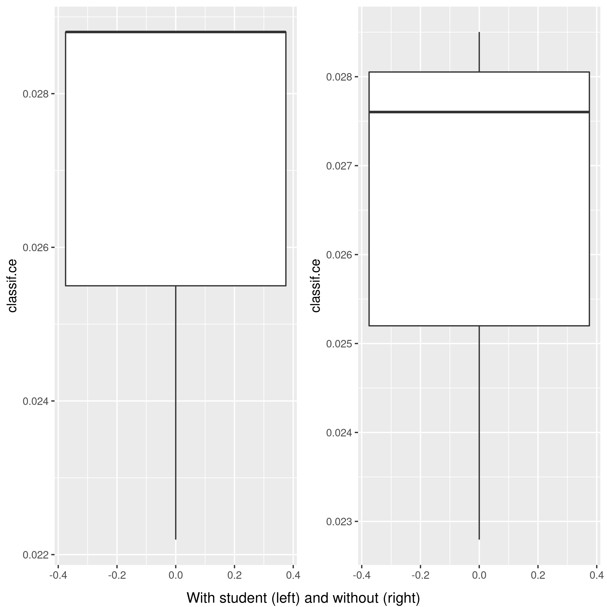
Figure 9: Plot of accuracy
Given the results, it is fair to say that adding the student data is useful in general.
Question 5.6 - Page 199
We continue to consider the use of a logistic regression model to
predict the probability of default using income and balance on the
Default data set. In particular, we will now compute estimates for the
standard errors of the income and balance logistic regression
coefficients in two different ways: (1) using the bootstrap, and (2)
using the standard formula for computing the standard errors in the
glm() function. Do not forget to set a random seed before beginning
your analysis.
(a) Using the summary() and glm() functions, determine the
estimated standard errors for the coefficients associated with income
and balance in a multiple logistic regression model that uses both
predictors.
(b) Write a function, boot.fn() , that takes as input the Default
data set as well as an index of the observations, and that outputs the
coefficient estimates for income and balance in the multiple
logistic regression model.
(c) Use the boot() function together with your boot.fn() function
to estimate the standard errors of the logistic regression coefficients
for income and balance.
(d) Comment on the estimated standard errors obtained using the
glm() function and using your bootstrap function.
Answer
This question is slightly more specific to the packages in the book so we will use them.
a) Fit summary
1glm.fit %>% summary
 1##
 2## Call:
 3## glm(formula = default ~ income + balance, family = binomial,
 4##     data = defDat, subset = trainNoCaret)
 5##
 6## Deviance Residuals:
 7##     Min       1Q   Median       3Q      Max
 8## -2.1943  -0.1488  -0.0588  -0.0217   3.7058
 9##
10## Coefficients:
11##               Estimate Std. Error z value Pr(>|z|)
12## (Intercept) -1.150e+01  4.814e-01 -23.885  < 2e-16 ***
13## income       2.288e-05  5.553e-06   4.121 3.78e-05 ***
14## balance      5.593e-03  2.509e-04  22.295  < 2e-16 ***
15## ---
16## Signif. codes:  0 '***' 0.001 '**' 0.01 '*' 0.05 '.' 0.1 ' ' 1
17##
18## (Dispersion parameter for binomial family taken to be 1)
19##
20##     Null deviance: 2354.0  on 7999  degrees of freedom
21## Residual deviance: 1283.6  on 7997  degrees of freedom
22## AIC: 1289.6
23##
24## Number of Fisher Scoring iterations: 8
b) Function
1boot.fn=function(data,subs){return(coef(glm(default~income+balance,data=data, family=binomial,subset=subs)))}
1boot.fn(defDat,train_set) %>% print
1##   (Intercept)        income       balance
2## -1.136824e+01  1.846153e-05  5.576468e-03
1glm(default~income+balance,data=defDat,family=binomial,subset=train_set) %>% summary
 1##
 2## Call:
 3## glm(formula = default ~ income + balance, family = binomial,
 4##     data = defDat, subset = train_set)
 5##
 6## Deviance Residuals:
 7##     Min       1Q   Median       3Q      Max
 8## -2.4280  -0.1465  -0.0582  -0.0218   3.7115
 9##
10## Coefficients:
11##               Estimate Std. Error z value Pr(>|z|)
12## (Intercept) -1.137e+01  4.813e-01 -23.618  < 2e-16 ***
13## income       1.846e-05  5.553e-06   3.324 0.000886 ***
14## balance      5.576e-03  2.529e-04  22.046  < 2e-16 ***
15## ---
16## Signif. codes:  0 '***' 0.001 '**' 0.01 '*' 0.05 '.' 0.1 ' ' 1
17##
18## (Dispersion parameter for binomial family taken to be 1)
19##
20##     Null deviance: 2313.6  on 7999  degrees of freedom
21## Residual deviance: 1266.4  on 7997  degrees of freedom
22## AIC: 1272.4
23##
24## Number of Fisher Scoring iterations: 8
We see that the statistics obtained from both are the same.
c) Bootstrap
The old fashioned way. R is the resample rate, boot.fn is the
statistic used.
1library(boot)
1##
2## Attaching package: 'boot'
1## The following object is masked from 'package:lattice':
2##
3##     melanoma
1boot(defDat,boot.fn,R=184) %>% print
 1##
 2## ORDINARY NONPARAMETRIC BOOTSTRAP
 3##
 4##
 5## Call:
 6## boot(data = defDat, statistic = boot.fn, R = 184)
 7##
 8##
 9## Bootstrap Statistics :
10##          original        bias     std. error
11## t1* -1.154047e+01 -1.407368e-02 4.073453e-01
12## t2*  2.080898e-05 -6.386634e-08 4.720109e-06
13## t3*  5.647103e-03  1.350950e-05 2.111547e-04
d) Comparison
- Clearly, there is not much difference in the standard error estimates
Var | Bootstrap | Summary |
| :———: | ——— |
Intercept | 4.428026e-01 | 4.883e-01 |
income | 2.797011e-06 | 5.548e-06 |
balance | 2.423002e-04 | 2.591e-04 |
Question 5.8 - Page 200
We will now perform cross-validation on a simulated data set. (a) Generate a simulated data set as follows:
1> set . seed (1)
2> y = rnorm (100)
3> x = rnorm (100)
4> y =x -2\* x ^2+ rnorm (100)
In this data set, what is n and what is p? Write out the model used to generate the data in equation form.
(b) Create a scatterplot of \(X\) against \(Y\). Comment on what you find.
(c) Set a random seed, and then compute the LOOCV errors that result from fitting the following four models using least squares:
\(Y=\beta_0+\beta_1X+\eta\)
\(Y=\beta_0+\beta_1X+\beta_2X^2+\eta\)
\(Y=\beta_0+\beta_1X+\beta_2X^2+\beta_{3}X^{3}+\eta\)
\(Y=\beta_0+\beta_1X+\beta_2X^2+\beta_{3}X^{3}+\beta_{4}X^{4}+\eta\)
Note you may find it helpful to use the data.frame() function to
create a single data set containing both \(X\) and \(Y\).
(d) Repeat (c) using another random seed, and report your results. Are your results the same as what you got in (c)? Why?
(e) Which of the models in (c) had the smallest LOOCV error? Is this what you expected? Explain your answer.
(f) Comment on the statistical significance of the coefficient esti- mates that results from fitting each of the models in (c) using least squares. Do these results agree with the conclusions drawn based on the cross-validation results?
Answer
a) Modeling data
1set.seed(1)
2y <- rnorm(100)
3x <- rnorm(100)
4y <- x - 2*x^2 + rnorm(100)
Clearly:
- Our equation is \(y=x-2x^{2}+\epsilon\) where \(epsilon\) is normally distributed from 100 samples
- We have \(n=100\) observations
- \(p=2\) where \(p\) is the number of features
b) Visual inspection
1qplot(x,y)
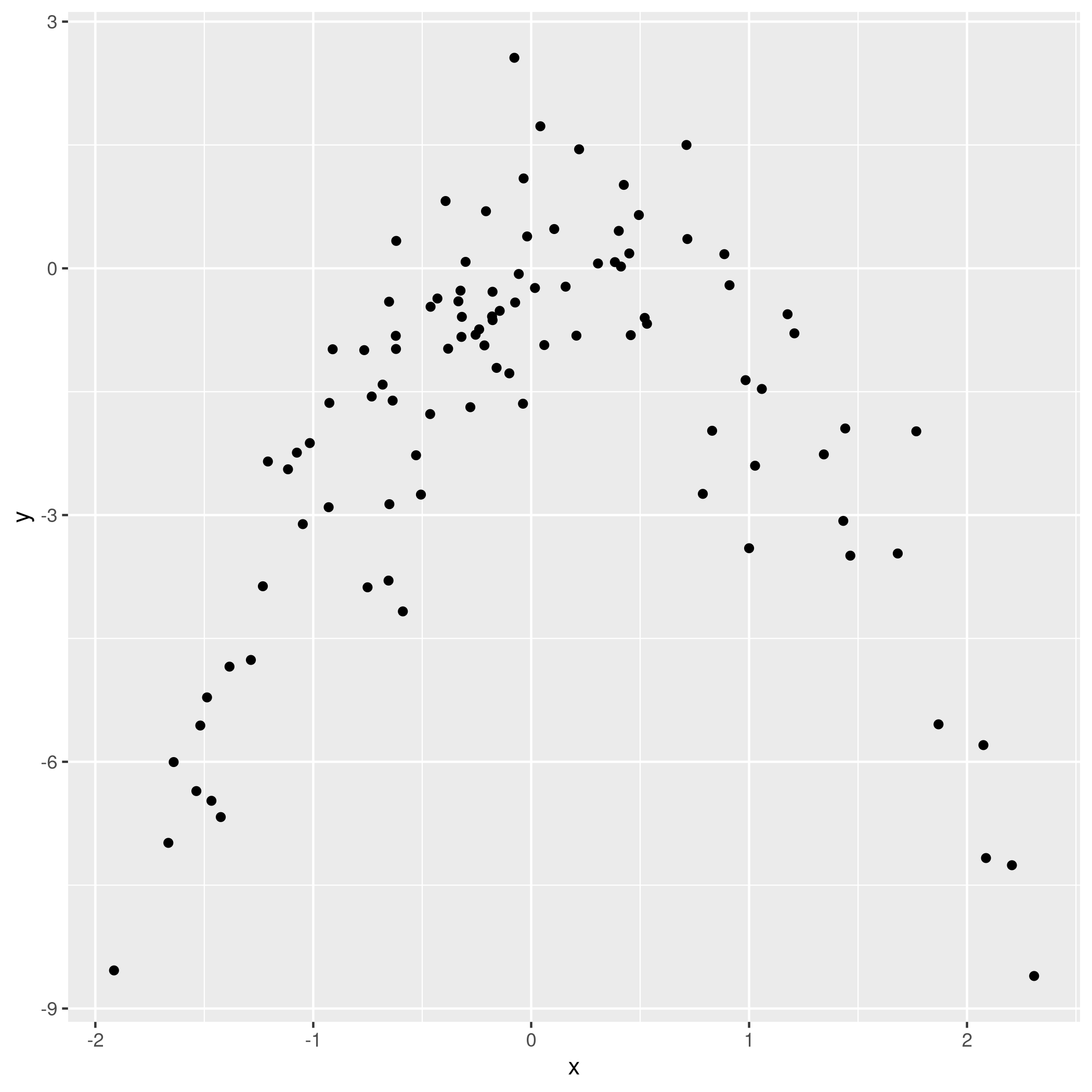
Figure 10: Model data plot
We observe that the data is quadratic, as we also know from the generating function, which was a quadratic equation plus normally distributed noise.
c) Least squares fits
Not very important, but here we use the caret form.
1pow=function(x,y){return(x^y)}
2dfDat <- data.frame(y,x,x2=pow(x,2),x3=pow(x,3),x4=pow(x,4))
We might have also just used poly(x,n) to skip making the data frame.
We will set our resampling method as follows:
1fitControl<-trainControl(method="LOOCV")
1train(y~x,data=dfDat,trControl=fitControl,method="lm") %>% print
 1## Linear Regression
 2##
 3## 100 samples
 4##   1 predictor
 5##
 6## No pre-processing
 7## Resampling: Leave-One-Out Cross-Validation
 8## Summary of sample sizes: 99, 99, 99, 99, 99, 99, ...
 9## Resampling results:
10##
11##   RMSE      Rsquared    MAE
12##   2.427134  0.05389864  1.878566
13##
14## Tuning parameter 'intercept' was held constant at a value of TRUE
1train(y~x+x2,data=dfDat,trControl=fitControl,method="lm") %>% print
 1## Linear Regression
 2##
 3## 100 samples
 4##   2 predictor
 5##
 6## No pre-processing
 7## Resampling: Leave-One-Out Cross-Validation
 8## Summary of sample sizes: 99, 99, 99, 99, 99, 99, ...
 9## Resampling results:
10##
11##   RMSE      Rsquared   MAE
12##   1.042399  0.8032414  0.8029942
13##
14## Tuning parameter 'intercept' was held constant at a value of TRUE
1train(y~x+x2+x3,data=dfDat,trControl=fitControl,method="lm") %>% print
 1## Linear Regression
 2##
 3## 100 samples
 4##   3 predictor
 5##
 6## No pre-processing
 7## Resampling: Leave-One-Out Cross-Validation
 8## Summary of sample sizes: 99, 99, 99, 99, 99, 99, ...
 9## Resampling results:
10##
11##   RMSE      Rsquared   MAE
12##   1.050041  0.8003517  0.8073024
13##
14## Tuning parameter 'intercept' was held constant at a value of TRUE
1train(y~x+x2+x3+x4,data=dfDat,trControl=fitControl,method="lm") %>% print
 1## Linear Regression
 2##
 3## 100 samples
 4##   4 predictor
 5##
 6## No pre-processing
 7## Resampling: Leave-One-Out Cross-Validation
 8## Summary of sample sizes: 99, 99, 99, 99, 99, 99, ...
 9## Resampling results:
10##
11##   RMSE      Rsquared   MAE
12##   1.055828  0.7982111  0.8150296
13##
14## Tuning parameter 'intercept' was held constant at a value of TRUE
d) Seeding effects
1set.seed(1995)
1train(y~x,data=dfDat,trControl=fitControl,method="lm") %>% print
 1## Linear Regression
 2##
 3## 100 samples
 4##   1 predictor
 5##
 6## No pre-processing
 7## Resampling: Leave-One-Out Cross-Validation
 8## Summary of sample sizes: 99, 99, 99, 99, 99, 99, ...
 9## Resampling results:
10##
11##   RMSE      Rsquared    MAE
12##   2.427134  0.05389864  1.878566
13##
14## Tuning parameter 'intercept' was held constant at a value of TRUE
1train(y~x+x2,data=dfDat,trControl=fitControl,method="lm") %>% print
 1## Linear Regression
 2##
 3## 100 samples
 4##   2 predictor
 5##
 6## No pre-processing
 7## Resampling: Leave-One-Out Cross-Validation
 8## Summary of sample sizes: 99, 99, 99, 99, 99, 99, ...
 9## Resampling results:
10##
11##   RMSE      Rsquared   MAE
12##   1.042399  0.8032414  0.8029942
13##
14## Tuning parameter 'intercept' was held constant at a value of TRUE
1train(y~x+x2+x3,data=dfDat,trControl=fitControl,method="lm") %>% print
 1## Linear Regression
 2##
 3## 100 samples
 4##   3 predictor
 5##
 6## No pre-processing
 7## Resampling: Leave-One-Out Cross-Validation
 8## Summary of sample sizes: 99, 99, 99, 99, 99, 99, ...
 9## Resampling results:
10##
11##   RMSE      Rsquared   MAE
12##   1.050041  0.8003517  0.8073024
13##
14## Tuning parameter 'intercept' was held constant at a value of TRUE
1train(y~x+x2+x3+x4,data=dfDat,trControl=fitControl,method="lm") %>% print
 1## Linear Regression
 2##
 3## 100 samples
 4##   4 predictor
 5##
 6## No pre-processing
 7## Resampling: Leave-One-Out Cross-Validation
 8## Summary of sample sizes: 99, 99, 99, 99, 99, 99, ...
 9## Resampling results:
10##
11##   RMSE      Rsquared   MAE
12##   1.055828  0.7982111  0.8150296
13##
14## Tuning parameter 'intercept' was held constant at a value of TRUE
We note that there is no change on varying the seed because LOOCV is exhaustive and uses n folds for each observation.
e) Analysis
1train(y~x,data=dfDat %>% subset(select=c(y,x)),trControl=fitControl,method="lm") %>% print
 1## Linear Regression
 2##
 3## 100 samples
 4##   1 predictor
 5##
 6## No pre-processing
 7## Resampling: Leave-One-Out Cross-Validation
 8## Summary of sample sizes: 99, 99, 99, 99, 99, 99, ...
 9## Resampling results:
10##
11##   RMSE      Rsquared    MAE
12##   2.427134  0.05389864  1.878566
13##
14## Tuning parameter 'intercept' was held constant at a value of TRUE
1train(y~poly(x,2),data=dfDat %>% subset(select=c(y,x)),trControl=fitControl,method="lm") %>% print
 1## Linear Regression
 2##
 3## 100 samples
 4##   1 predictor
 5##
 6## No pre-processing
 7## Resampling: Leave-One-Out Cross-Validation
 8## Summary of sample sizes: 99, 99, 99, 99, 99, 99, ...
 9## Resampling results:
10##
11##   RMSE      Rsquared   MAE
12##   1.042399  0.8032414  0.8029942
13##
14## Tuning parameter 'intercept' was held constant at a value of TRUE
1train(y~poly(x,3),data=dfDat %>% subset(select=c(y,x)),trControl=fitControl,method="lm") %>% print
 1## Linear Regression
 2##
 3## 100 samples
 4##   1 predictor
 5##
 6## No pre-processing
 7## Resampling: Leave-One-Out Cross-Validation
 8## Summary of sample sizes: 99, 99, 99, 99, 99, 99, ...
 9## Resampling results:
10##
11##   RMSE      Rsquared   MAE
12##   1.050041  0.8003517  0.8073024
13##
14## Tuning parameter 'intercept' was held constant at a value of TRUE
1train(y~poly(x,4),data=dfDat %>% subset(select=c(y,x)),trControl=fitControl,method="lm") %>% print
 1## Linear Regression
 2##
 3## 100 samples
 4##   1 predictor
 5##
 6## No pre-processing
 7## Resampling: Leave-One-Out Cross-Validation
 8## Summary of sample sizes: 99, 99, 99, 99, 99, 99, ...
 9## Resampling results:
10##
11##   RMSE      Rsquared   MAE
12##   1.055828  0.7982111  0.8150296
13##
14## Tuning parameter 'intercept' was held constant at a value of TRUE
Clearly the quadratic polynomial has the lowest error, which makes sense given how the data was generated.
f) Statistical significance
1train(y~x,data=dfDat %>% subset(select=c(y,x)),trControl=fitControl,method="lm") %>% summary %>% print
 1##
 2## Call:
 3## lm(formula = .outcome ~ ., data = dat)
 4##
 5## Residuals:
 6##     Min      1Q  Median      3Q     Max
 7## -7.3469 -0.9275  0.8028  1.5608  4.3974
 8##
 9## Coefficients:
10##             Estimate Std. Error t value Pr(>|t|)
11## (Intercept)  -1.8185     0.2364  -7.692 1.14e-11 ***
12## x             0.2430     0.2479   0.981    0.329
13## ---
14## Signif. codes:  0 '***' 0.001 '**' 0.01 '*' 0.05 '.' 0.1 ' ' 1
15##
16## Residual standard error: 2.362 on 98 degrees of freedom
17## Multiple R-squared:  0.009717,   Adjusted R-squared:  -0.0003881
18## F-statistic: 0.9616 on 1 and 98 DF,  p-value: 0.3292
1train(y~poly(x,2),data=dfDat %>% subset(select=c(y,x)),trControl=fitControl,method="lm") %>% summary %>% print
 1##
 2## Call:
 3## lm(formula = .outcome ~ ., data = dat)
 4##
 5## Residuals:
 6##      Min       1Q   Median       3Q      Max
 7## -2.89884 -0.53765  0.04135  0.61490  2.73607
 8##
 9## Coefficients:
10##               Estimate Std. Error t value Pr(>|t|)
11## (Intercept)    -1.8277     0.1032 -17.704   <2e-16 ***
12## `poly(x, 2)1`   2.3164     1.0324   2.244   0.0271 *
13## `poly(x, 2)2` -21.0586     1.0324 -20.399   <2e-16 ***
14## ---
15## Signif. codes:  0 '***' 0.001 '**' 0.01 '*' 0.05 '.' 0.1 ' ' 1
16##
17## Residual standard error: 1.032 on 97 degrees of freedom
18## Multiple R-squared:  0.8128, Adjusted R-squared:  0.8089
19## F-statistic: 210.6 on 2 and 97 DF,  p-value: < 2.2e-16
1train(y~poly(x,3),data=dfDat %>% subset(select=c(y,x)),trControl=fitControl,method="lm") %>% summary %>% print
 1##
 2## Call:
 3## lm(formula = .outcome ~ ., data = dat)
 4##
 5## Residuals:
 6##      Min       1Q   Median       3Q      Max
 7## -2.87250 -0.53881  0.02862  0.59383  2.74350
 8##
 9## Coefficients:
10##               Estimate Std. Error t value Pr(>|t|)
11## (Intercept)    -1.8277     0.1037 -17.621   <2e-16 ***
12## `poly(x, 3)1`   2.3164     1.0372   2.233   0.0279 *
13## `poly(x, 3)2` -21.0586     1.0372 -20.302   <2e-16 ***
14## `poly(x, 3)3`  -0.3048     1.0372  -0.294   0.7695
15## ---
16## Signif. codes:  0 '***' 0.001 '**' 0.01 '*' 0.05 '.' 0.1 ' ' 1
17##
18## Residual standard error: 1.037 on 96 degrees of freedom
19## Multiple R-squared:  0.813,  Adjusted R-squared:  0.8071
20## F-statistic: 139.1 on 3 and 96 DF,  p-value: < 2.2e-16
1train(y~poly(x,4),data=dfDat %>% subset(select=c(y,x)),trControl=fitControl,method="lm") %>% summary %>% print
 1##
 2## Call:
 3## lm(formula = .outcome ~ ., data = dat)
 4##
 5## Residuals:
 6##     Min      1Q  Median      3Q     Max
 7## -2.8914 -0.5244  0.0749  0.5932  2.7796
 8##
 9## Coefficients:
10##               Estimate Std. Error t value Pr(>|t|)
11## (Intercept)    -1.8277     0.1041 -17.549   <2e-16 ***
12## `poly(x, 4)1`   2.3164     1.0415   2.224   0.0285 *
13## `poly(x, 4)2` -21.0586     1.0415 -20.220   <2e-16 ***
14## `poly(x, 4)3`  -0.3048     1.0415  -0.293   0.7704
15## `poly(x, 4)4`  -0.4926     1.0415  -0.473   0.6373
16## ---
17## Signif. codes:  0 '***' 0.001 '**' 0.01 '*' 0.05 '.' 0.1 ' ' 1
18##
19## Residual standard error: 1.041 on 95 degrees of freedom
20## Multiple R-squared:  0.8134, Adjusted R-squared:  0.8055
21## F-statistic: 103.5 on 4 and 95 DF,  p-value: < 2.2e-16
- Clearly, the second order terms are the most significant, as expected
Question 5.9 - Page 201
We will now consider the Boston housing data set, from the MASS library.
(a) Based on this data set, provide an estimate for the population
mean of medv. Call this estimate \(\hat{\mu}\).
(b) Provide an estimate of the standard error of \(\hat{\mu}\). Interpret this result. Hint: We can compute the standard error of the sample mean by dividing the sample standard deviation by the square root of the number of observations.
(c) Now estimate the standard error of \(\hat{\mu}\) using the bootstrap. How does this compare to your answer from (b)?
(d) Based on your bootstrap estimate from (c), provide a 95 %
confidence interval for the mean of medv. Compare it to the results
obtained using t.test(Boston\$medv). Hint: You can approximate a 95 %
confidence interval using the formula
\([\hat{\mu} − 2SE(\hat{\mu}), \hat{\mu} + 2SE(\hat{\mu})]\).
(e) Based on this data set, provide an estimate, \(\hat{\mu_{med}}\),
for the median value of medv in the population.
(f) We now would like to estimate the standard error of \(\hat{\mu}\) med. Unfortunately, there is no simple formula for computing the standard error of the median. Instead, estimate the standard error of the median using the bootstrap. Comment on your findings.
(g) Based on this data set, provide an estimate for the tenth
percentile of medv in Boston suburbs. Call this quantity
\(\hat{\mu_{0.1}}\). (You can use the quantile() function.)
(h) Use the bootstrap to estimate the standard error of \(\hat{\mu_{0.1}}\). Comment on your findings.
Answer
1boston<-MASS::Boston
- Reminder
1boston %>% summary %>% print
 1##       crim                zn             indus            chas
 2##  Min.   : 0.00632   Min.   :  0.00   Min.   : 0.46   Min.   :0.00000
 3##  1st Qu.: 0.08204   1st Qu.:  0.00   1st Qu.: 5.19   1st Qu.:0.00000
 4##  Median : 0.25651   Median :  0.00   Median : 9.69   Median :0.00000
 5##  Mean   : 3.61352   Mean   : 11.36   Mean   :11.14   Mean   :0.06917
 6##  3rd Qu.: 3.67708   3rd Qu.: 12.50   3rd Qu.:18.10   3rd Qu.:0.00000
 7##  Max.   :88.97620   Max.   :100.00   Max.   :27.74   Max.   :1.00000
 8##       nox               rm             age              dis
 9##  Min.   :0.3850   Min.   :3.561   Min.   :  2.90   Min.   : 1.130
10##  1st Qu.:0.4490   1st Qu.:5.886   1st Qu.: 45.02   1st Qu.: 2.100
11##  Median :0.5380   Median :6.208   Median : 77.50   Median : 3.207
12##  Mean   :0.5547   Mean   :6.285   Mean   : 68.57   Mean   : 3.795
13##  3rd Qu.:0.6240   3rd Qu.:6.623   3rd Qu.: 94.08   3rd Qu.: 5.188
14##  Max.   :0.8710   Max.   :8.780   Max.   :100.00   Max.   :12.127
15##       rad              tax           ptratio          black
16##  Min.   : 1.000   Min.   :187.0   Min.   :12.60   Min.   :  0.32
17##  1st Qu.: 4.000   1st Qu.:279.0   1st Qu.:17.40   1st Qu.:375.38
18##  Median : 5.000   Median :330.0   Median :19.05   Median :391.44
19##  Mean   : 9.549   Mean   :408.2   Mean   :18.46   Mean   :356.67
20##  3rd Qu.:24.000   3rd Qu.:666.0   3rd Qu.:20.20   3rd Qu.:396.23
21##  Max.   :24.000   Max.   :711.0   Max.   :22.00   Max.   :396.90
22##      lstat            medv
23##  Min.   : 1.73   Min.   : 5.00
24##  1st Qu.: 6.95   1st Qu.:17.02
25##  Median :11.36   Median :21.20
26##  Mean   :12.65   Mean   :22.53
27##  3rd Qu.:16.95   3rd Qu.:25.00
28##  Max.   :37.97   Max.   :50.00
1boston %>% str %>% print
 1## 'data.frame':    506 obs. of  14 variables:
 2##  $ crim   : num  0.00632 0.02731 0.02729 0.03237 0.06905 ...
 3##  $ zn     : num  18 0 0 0 0 0 12.5 12.5 12.5 12.5 ...
 4##  $ indus  : num  2.31 7.07 7.07 2.18 2.18 2.18 7.87 7.87 7.87 7.87 ...
 5##  $ chas   : int  0 0 0 0 0 0 0 0 0 0 ...
 6##  $ nox    : num  0.538 0.469 0.469 0.458 0.458 0.458 0.524 0.524 0.524 0.524 ...
 7##  $ rm     : num  6.58 6.42 7.18 7 7.15 ...
 8##  $ age    : num  65.2 78.9 61.1 45.8 54.2 58.7 66.6 96.1 100 85.9 ...
 9##  $ dis    : num  4.09 4.97 4.97 6.06 6.06 ...
10##  $ rad    : int  1 2 2 3 3 3 5 5 5 5 ...
11##  $ tax    : num  296 242 242 222 222 222 311 311 311 311 ...
12##  $ ptratio: num  15.3 17.8 17.8 18.7 18.7 18.7 15.2 15.2 15.2 15.2 ...
13##  $ black  : num  397 397 393 395 397 ...
14##  $ lstat  : num  4.98 9.14 4.03 2.94 5.33 ...
15##  $ medv   : num  24 21.6 34.7 33.4 36.2 28.7 22.9 27.1 16.5 18.9 ...
16## NULL
a) Mean
1muhat=boston$medv %>% mean()
2print(muhat)
1## [1] 22.53281
b) Standard error
Recall that \(SE=\frac{SD}{\sqrt{N_{obs}}}\)
1boston$medv %>% sd/(nrow(boston)^0.5) %>% print
1## [1] 22.49444
1## [1] 0.4088611
c) Bootstrap estimate
1library(boot)
2myMean<-function(frame,ind){return(mean(frame[ind]))}
1boot(boston$medv,myMean,R=184) %>% print
 1##
 2## ORDINARY NONPARAMETRIC BOOTSTRAP
 3##
 4##
 5## Call:
 6## boot(data = boston$medv, statistic = myMean, R = 184)
 7##
 8##
 9## Bootstrap Statistics :
10##     original     bias    std. error
11## t1* 22.53281 0.03451839    0.409621
We see that the bootstrapped error over 184 samples is 0.4341499 while
without it we had 0.4088611 which is similar enough.
d) Confidence intervals with bootstrap and t.test
1boston$medv %>% t.test %>% print
 1##
 2##  One Sample t-test
 3##
 4## data:  .
 5## t = 55.111, df = 505, p-value < 2.2e-16
 6## alternative hypothesis: true mean is not equal to 0
 7## 95 percent confidence interval:
 8##  21.72953 23.33608
 9## sample estimates:
10## mean of x
11##  22.53281
We can approximate this with what we already have
1bRes=boot(boston$medv,myMean,R=184)
2seBoot<-bRes$t %>% var %>% sqrt
3xlow=muhat-2*(seBoot)
4xhigh=muhat+2*(seBoot)
5c(xlow,xhigh) %>% print
1## [1] 21.72675 23.33887
Our intervals are also pretty close to each other.
e) Median
1boston$medv %>% sort %>% median %>% print
1## [1] 21.2
f) Median standard error
We can reuse the logic of the myMean function defined previously.
1myMedian=function(data,ind){return(median(data[ind]))}
1boston$medv %>% boot(myMedian,R=1500) %>% print
 1##
 2## ORDINARY NONPARAMETRIC BOOTSTRAP
 3##
 4##
 5## Call:
 6## boot(data = ., statistic = myMedian, R = 1500)
 7##
 8##
 9## Bootstrap Statistics :
10##     original      bias    std. error
11## t1*     21.2 -0.03773333    0.387315
We see that the standard error is 0.3767072.
g) Tenth percentile
1mu0one<-boston$medv %>% quantile(c(0.1))
2print(mu0one)
1##   10%
2## 12.75
h) Bootstrap
Once again.
1myQuant=function(data,ind){return(quantile(data[ind],0.1))}
1boston$medv %>% boot(myQuant,R=500) %>% print
 1##
 2## ORDINARY NONPARAMETRIC BOOTSTRAP
 3##
 4##
 5## Call:
 6## boot(data = ., statistic = myQuant, R = 500)
 7##
 8##
 9## Bootstrap Statistics :
10##     original  bias    std. error
11## t1*    12.75 -0.0095   0.4951415
The standard error is 0.5024526
James, G., Witten, D., Hastie, T., & Tibshirani, R. (2013). An Introduction to Statistical Learning: with Applications in R. Berlin, Germany: Springer Science & Business Media. ↩︎
Lang et al., (2019). mlr3: A modern object-oriented machine learning framework in R. Journal of Open Source Software, 4(44), 1903, https://doi.org/10.21105/joss.01903 ↩︎
![]()