
57 minutes
Written: 2020-02-19 07:00 +0000
ISLR :: Linear Model Selection and Regularization
Chapter VI - Linear Model Selection and Regularization
All the questions are as per the ISL seventh printing of the First edition1.
Common
Instead of using the standard functions, we will leverage the mlr3
package2.
1#install.packages("mlr3","data.table","mlr3viz","mlr3learners")
Actually for R version 3.6.2, the steps to get it working were a bit
more involved.
Load ISLR and other libraries.
1libsUsed<-c("dplyr","ggplot2","tidyverse",
2            "ISLR","caret","MASS", "gridExtra",
3            "pls","latex2exp","data.table")
4invisible(lapply(libsUsed, library, character.only = TRUE))
Question 6.8 - Page 262
In this exercise, we will generate simulated data, and will then use this data to perform best subset selection.
(a) Use the =rnorm()=function to generate a predictor \(X\) of length \(n = 100\), as well as a noise vector \(\eta\) of length \(n = 100\).
(b) Generate a response vector \(Y\) of length \(n = 100\) according to the model \[Y = \beta_0 + \beta_1X + \beta2X^2 + \beta_3X^3 + \eta\], where \(\beta_{0}\) , \(\beta_{1}\), \(\beta_{2}\), and \(\beta_{3}\) are constants of your choice.
(c) Use the regsubsets() function to perform best subset selection
in order to choose the best model containing the predictors \(X\),
\(X^{2}\), …, \(X^{10}\). What is the best model obtained according to
\(C_p\) , BIC, and adjusted \(R^2\) ? Show some plots to provide evidence
for your answer, and report the coefficients of the best model obtained.
Note you will need to use the data.frame() function to create a single
data set containing both \(X\) and \(Y\).
(d) Repeat (c), using forward stepwise selection and also using backwards stepwise selection. How does your answer compare to the results in (c)?
(e) Now fit a lasso model to the simulated data, again using \(X\), \(X^{2}\), …, \(X^{10}\) as predictors. Use cross-validation to select the optimal value of \(\lambda\). Create plots of the cross-validation error as a function of \(\lambda\). Report the resulting coefficient estimates, and discuss the results obtained.
(f) Now generate a response vector Y according to the model \[Y = \beta_{0} + \beta_{7}X^{7} + \eta,\] and perform best subset selection and the lasso. Discuss the results obtained.
Answer
a) Generate model
1set.seed(1984)
2x<-rnorm(100)
3noise<-rnorm(100)
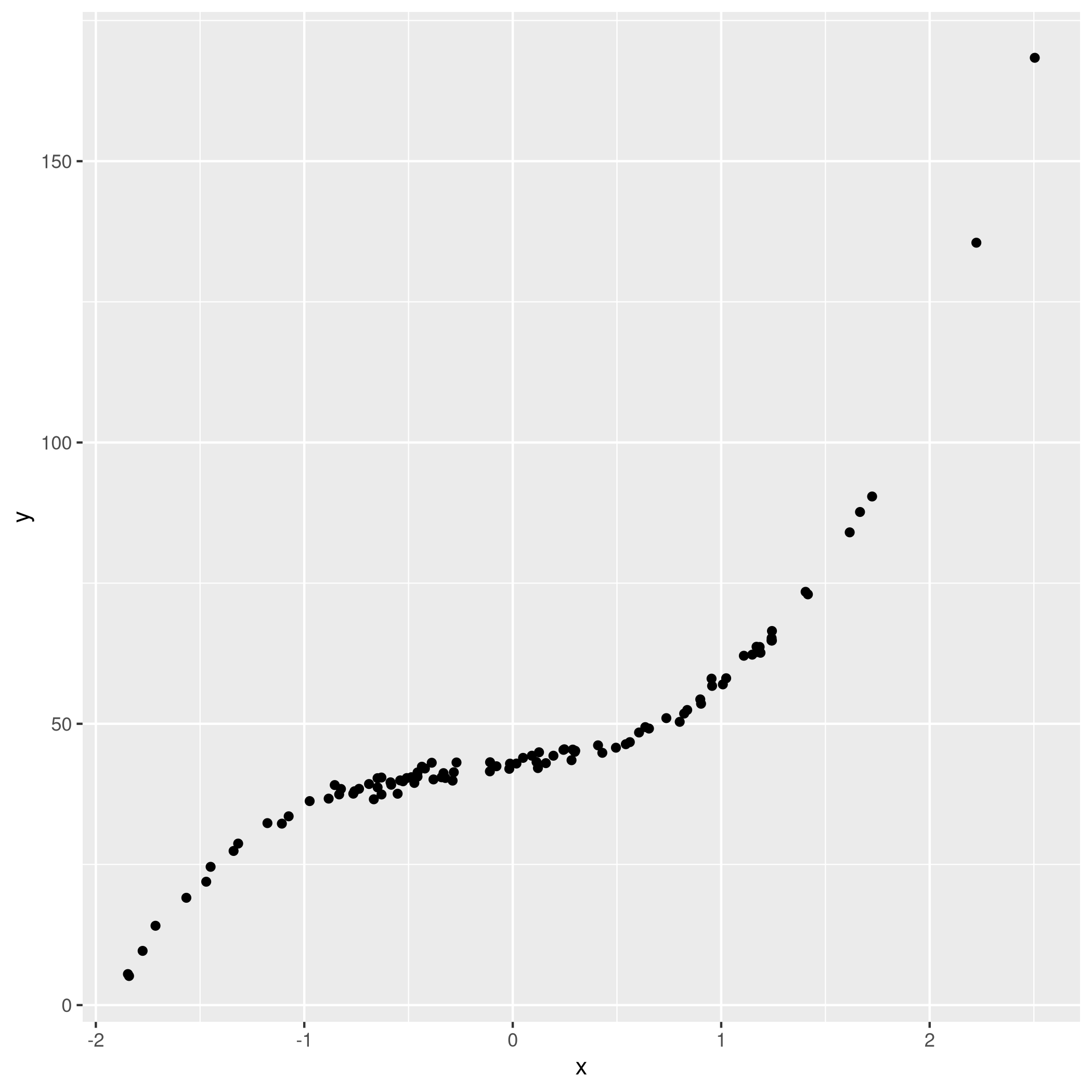
b) Response vector
1beta=c(43,5,3,6)
2y<-beta[1] + beta[2]*x + beta[3]*x^2 + beta[4]*x^3 + noise
3qplot(x,y)
c) Subset selection
Since the question requires it, we will be using the leaps libraries.
1library(leaps)
2df<-data.frame(y=y,x=x)
3sets=regsubsets(y~poly(x,10,raw=T),data=df,nvmax=10)
4sets %>% summary
 1## Subset selection object
 2## Call: regsubsets.formula(y ~ poly(x, 10, raw = T), data = df, nvmax = 10)
 3## 10 Variables  (and intercept)
 4##                        Forced in Forced out
 5## poly(x, 10, raw = T)1      FALSE      FALSE
 6## poly(x, 10, raw = T)2      FALSE      FALSE
 7## poly(x, 10, raw = T)3      FALSE      FALSE
 8## poly(x, 10, raw = T)4      FALSE      FALSE
 9## poly(x, 10, raw = T)5      FALSE      FALSE
10## poly(x, 10, raw = T)6      FALSE      FALSE
11## poly(x, 10, raw = T)7      FALSE      FALSE
12## poly(x, 10, raw = T)8      FALSE      FALSE
13## poly(x, 10, raw = T)9      FALSE      FALSE
14## poly(x, 10, raw = T)10     FALSE      FALSE
15## 1 subsets of each size up to 10
16## Selection Algorithm: exhaustive
17##           poly(x, 10, raw = T)1 poly(x, 10, raw = T)2 poly(x, 10, raw = T)3
18## 1  ( 1 )  " "                   " "                   "*"
19## 2  ( 1 )  " "                   "*"                   "*"
20## 3  ( 1 )  "*"                   "*"                   "*"
21## 4  ( 1 )  "*"                   "*"                   "*"
22## 5  ( 1 )  "*"                   "*"                   "*"
23## 6  ( 1 )  "*"                   " "                   "*"
24## 7  ( 1 )  "*"                   "*"                   "*"
25## 8  ( 1 )  "*"                   "*"                   "*"
26## 9  ( 1 )  "*"                   "*"                   "*"
27## 10  ( 1 ) "*"                   "*"                   "*"
28##           poly(x, 10, raw = T)4 poly(x, 10, raw = T)5 poly(x, 10, raw = T)6
29## 1  ( 1 )  " "                   " "                   " "
30## 2  ( 1 )  " "                   " "                   " "
31## 3  ( 1 )  " "                   " "                   " "
32## 4  ( 1 )  "*"                   " "                   " "
33## 5  ( 1 )  " "                   " "                   " "
34## 6  ( 1 )  "*"                   " "                   "*"
35## 7  ( 1 )  "*"                   " "                   "*"
36## 8  ( 1 )  "*"                   "*"                   "*"
37## 9  ( 1 )  "*"                   " "                   "*"
38## 10  ( 1 ) "*"                   "*"                   "*"
39##           poly(x, 10, raw = T)7 poly(x, 10, raw = T)8 poly(x, 10, raw = T)9
40## 1  ( 1 )  " "                   " "                   " "
41## 2  ( 1 )  " "                   " "                   " "
42## 3  ( 1 )  " "                   " "                   " "
43## 4  ( 1 )  " "                   " "                   " "
44## 5  ( 1 )  " "                   " "                   "*"
45## 6  ( 1 )  " "                   "*"                   " "
46## 7  ( 1 )  " "                   "*"                   " "
47## 8  ( 1 )  " "                   "*"                   " "
48## 9  ( 1 )  "*"                   "*"                   "*"
49## 10  ( 1 ) "*"                   "*"                   "*"
50##           poly(x, 10, raw = T)10
51## 1  ( 1 )  " "
52## 2  ( 1 )  " "
53## 3  ( 1 )  " "
54## 4  ( 1 )  " "
55## 5  ( 1 )  "*"
56## 6  ( 1 )  "*"
57## 7  ( 1 )  "*"
58## 8  ( 1 )  "*"
59## 9  ( 1 )  "*"
60## 10  ( 1 ) "*"
We also want the best parameters.
1summarySet<-summary(sets)
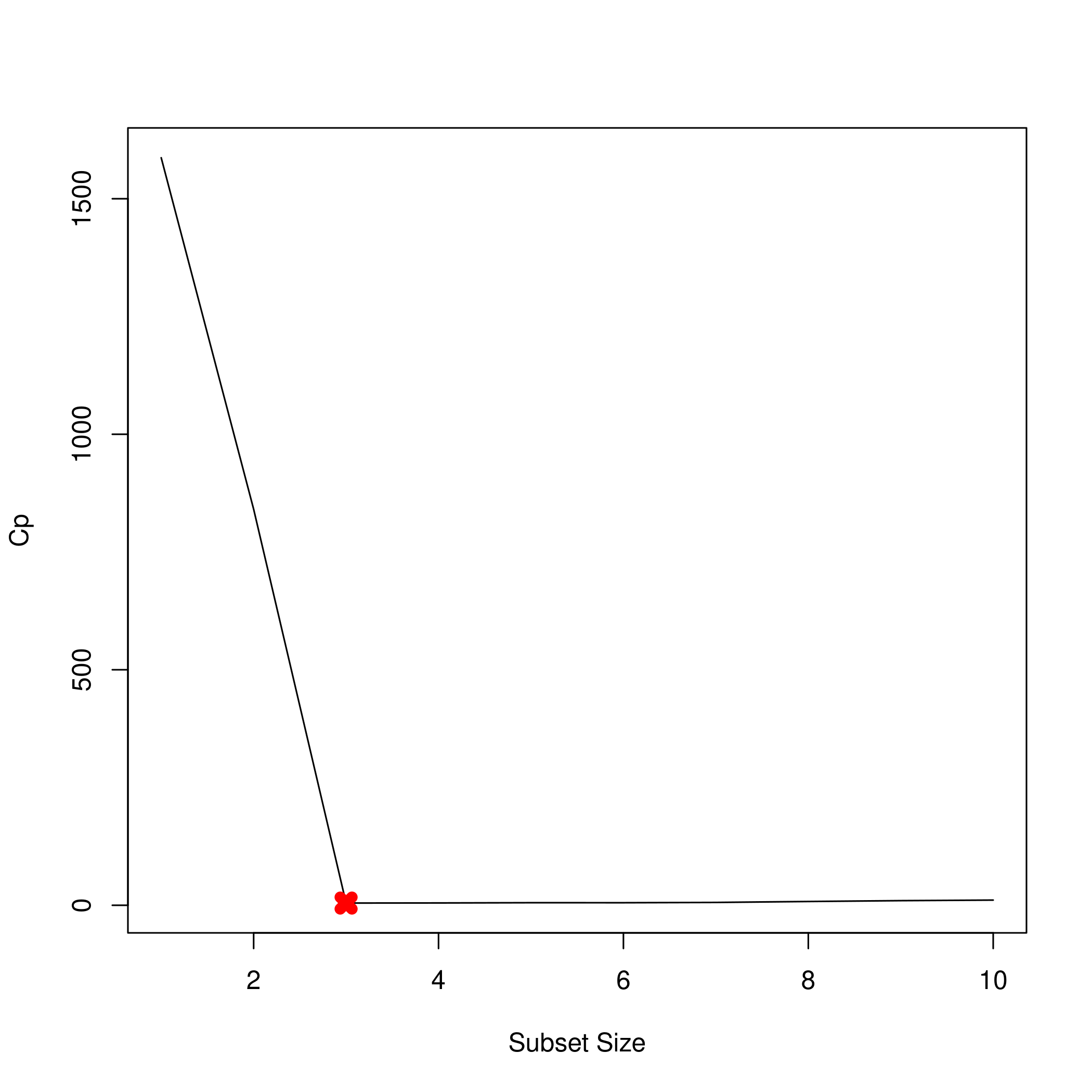
2which.min(summarySet$cp) %>% print
1## [1] 3
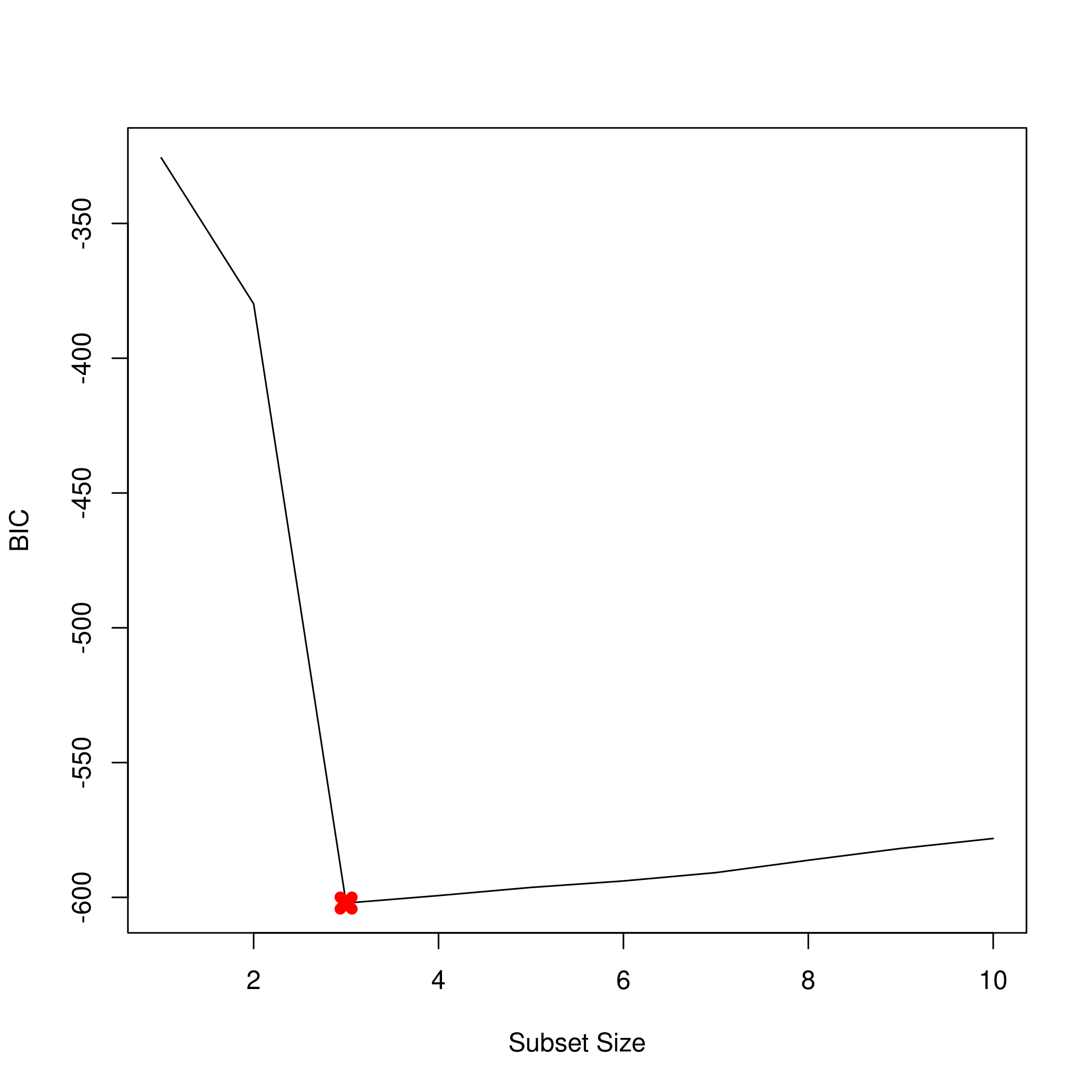
1which.min(summarySet$bic) %>% print
1## [1] 3
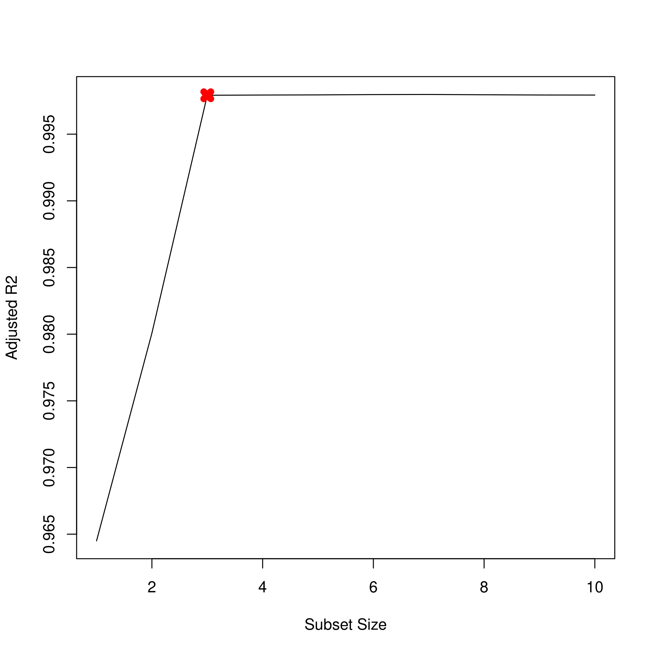
1which.max(summarySet$adjr2) %>% print
1## [1] 7
We might want to see this as a plot.
1plot(summarySet$cp, xlab = "Subset Size", ylab = "Cp", pch = 20, type = "l")
2points(3,summarySet$cp[3],pch=4,col='red',lwd=7)
1plot(summarySet$bic, xlab = "Subset Size", ylab = "BIC", pch = 20, type = "l")
2points(3,summarySet$bic[3],pch=4,col='red',lwd=7)
1plot(summarySet$adjr2, xlab = "Subset Size", ylab = "Adjusted R2", pch = 20, type = "l")
2points(3,summarySet$adjr2[3],pch=4,col='red',lwd=7)
Lets check the coefficients.
1coefficients(sets,id=3) %>% print
1##           (Intercept) poly(x, 10, raw = T)1 poly(x, 10, raw = T)2
2##             42.895657              5.108094              3.034408
3## poly(x, 10, raw = T)3
4##              5.989367
1beta %>% print
1## [1] 43 5 3 6
We see that we actually have a pretty good set of coefficients.
d) Forward and backward stepwise models
1modelX<-poly(x,10,raw=T)
2forwardFit<-regsubsets(y~modelX,data=df,nvmax=10,method="forward")
3forwardFit %>% summary %>% print
 1## Subset selection object
 2## Call: regsubsets.formula(y ~ modelX, data = df, nvmax = 10, method = "forward")
 3## 10 Variables  (and intercept)
 4##          Forced in Forced out
 5## modelX1      FALSE      FALSE
 6## modelX2      FALSE      FALSE
 7## modelX3      FALSE      FALSE
 8## modelX4      FALSE      FALSE
 9## modelX5      FALSE      FALSE
10## modelX6      FALSE      FALSE
11## modelX7      FALSE      FALSE
12## modelX8      FALSE      FALSE
13## modelX9      FALSE      FALSE
14## modelX10     FALSE      FALSE
15## 1 subsets of each size up to 10
16## Selection Algorithm: forward
17##           modelX1 modelX2 modelX3 modelX4 modelX5 modelX6 modelX7 modelX8
18## 1  ( 1 )  " "     " "     "*"     " "     " "     " "     " "     " "
19## 2  ( 1 )  " "     "*"     "*"     " "     " "     " "     " "     " "
20## 3  ( 1 )  "*"     "*"     "*"     " "     " "     " "     " "     " "
21## 4  ( 1 )  "*"     "*"     "*"     "*"     " "     " "     " "     " "
22## 5  ( 1 )  "*"     "*"     "*"     "*"     "*"     " "     " "     " "
23## 6  ( 1 )  "*"     "*"     "*"     "*"     "*"     " "     " "     " "
24## 7  ( 1 )  "*"     "*"     "*"     "*"     "*"     " "     "*"     " "
25## 8  ( 1 )  "*"     "*"     "*"     "*"     "*"     " "     "*"     "*"
26## 9  ( 1 )  "*"     "*"     "*"     "*"     "*"     "*"     "*"     "*"
27## 10  ( 1 ) "*"     "*"     "*"     "*"     "*"     "*"     "*"     "*"
28##           modelX9 modelX10
29## 1  ( 1 )  " "     " "
30## 2  ( 1 )  " "     " "
31## 3  ( 1 )  " "     " "
32## 4  ( 1 )  " "     " "
33## 5  ( 1 )  " "     " "
34## 6  ( 1 )  " "     "*"
35## 7  ( 1 )  " "     "*"
36## 8  ( 1 )  " "     "*"
37## 9  ( 1 )  " "     "*"
38## 10  ( 1 ) "*"     "*"
We might want to take a look at these.
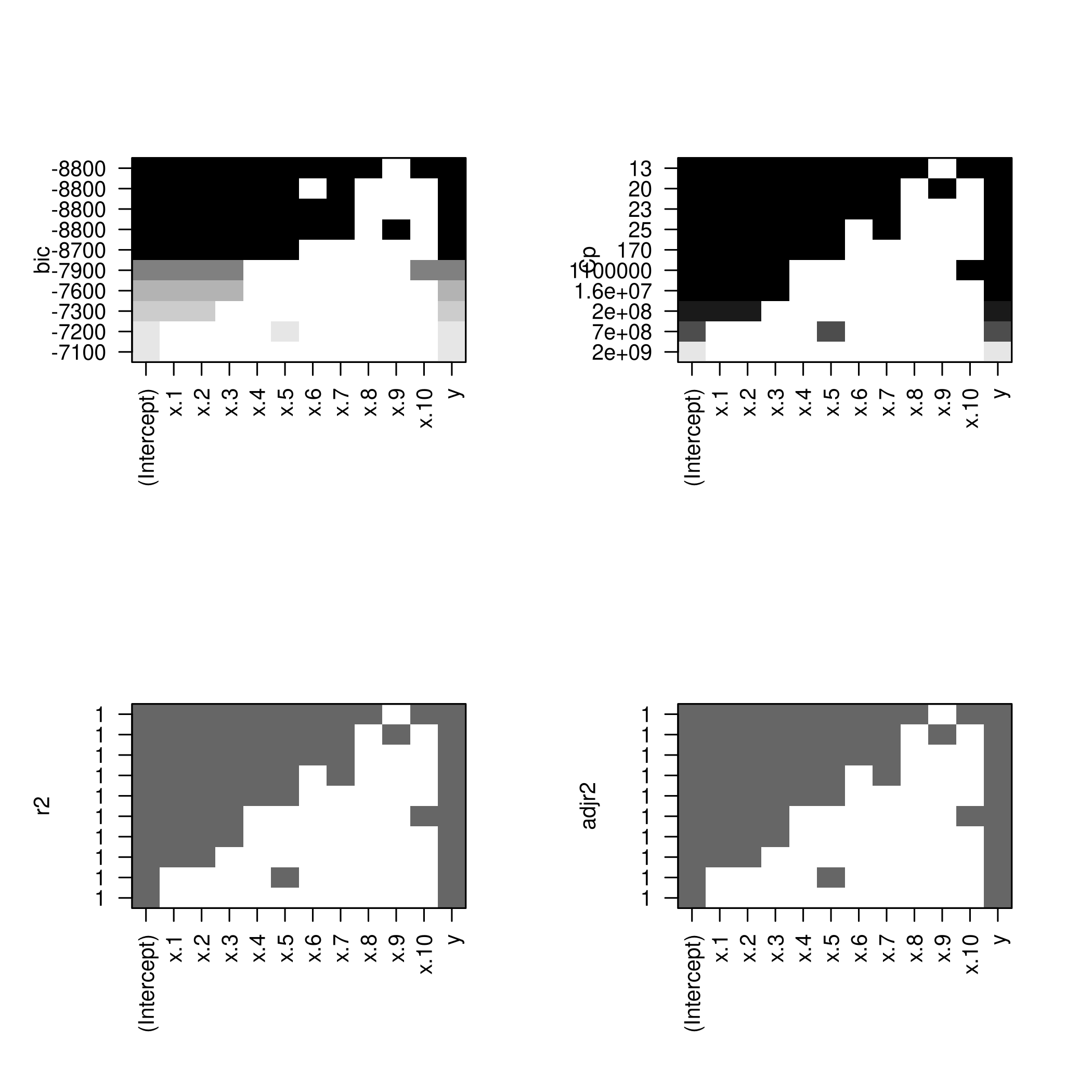
1par(mfrow=c(2,2))
2plot(forwardFit)
3plot(forwardFit,scale='Cp')
4plot(forwardFit,scale='r2')
5plot(forwardFit,scale='adjr2')
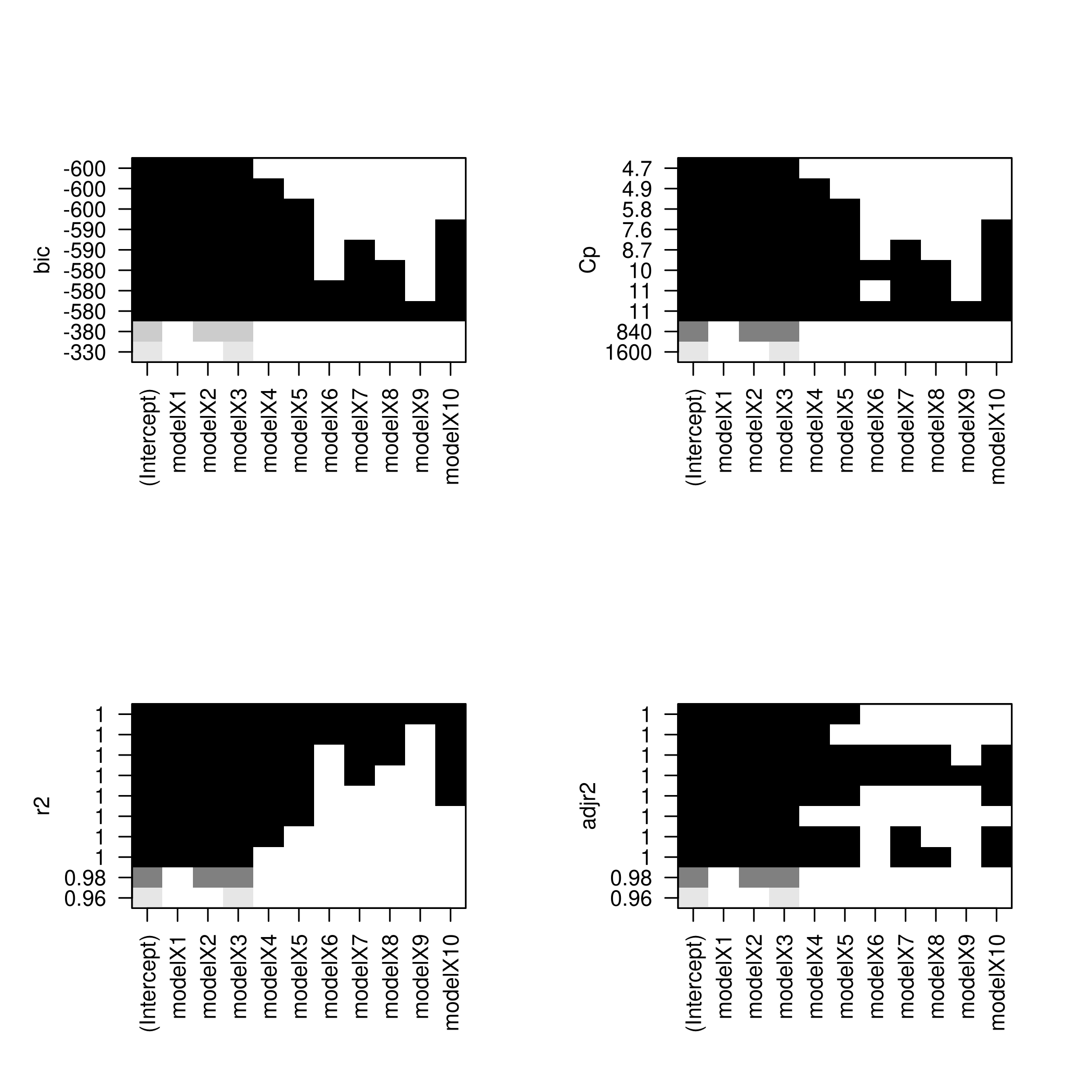
I find these not as fun to look at, so we will do better.
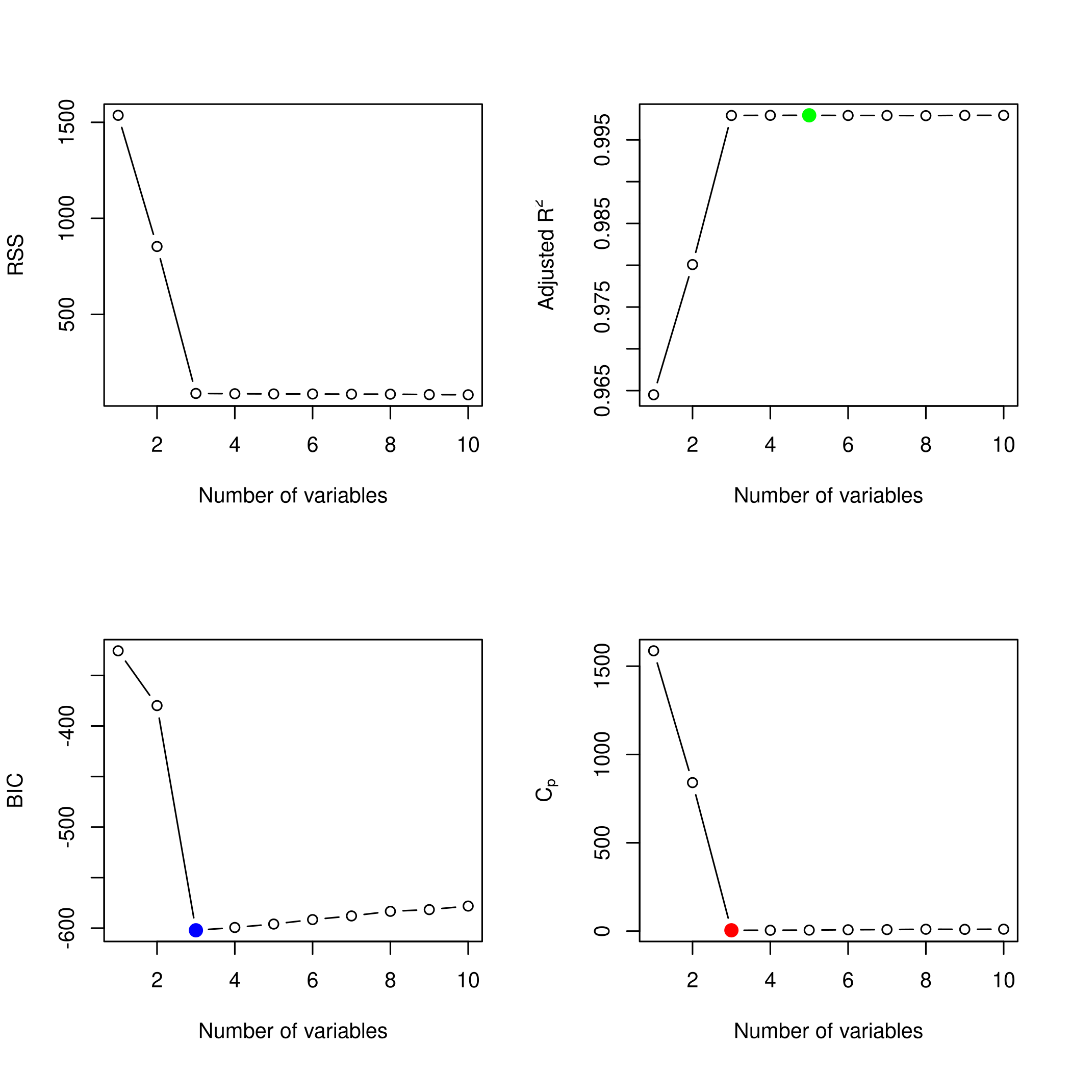
1plotLEAP=function(leapObj){
2 par(mfrow = c(2,2))
3 bar2=which.max(leapObj$adjr2)
4 bbic=which.min(leapObj$bic)
5 bcp=which.min(leapObj$cp)
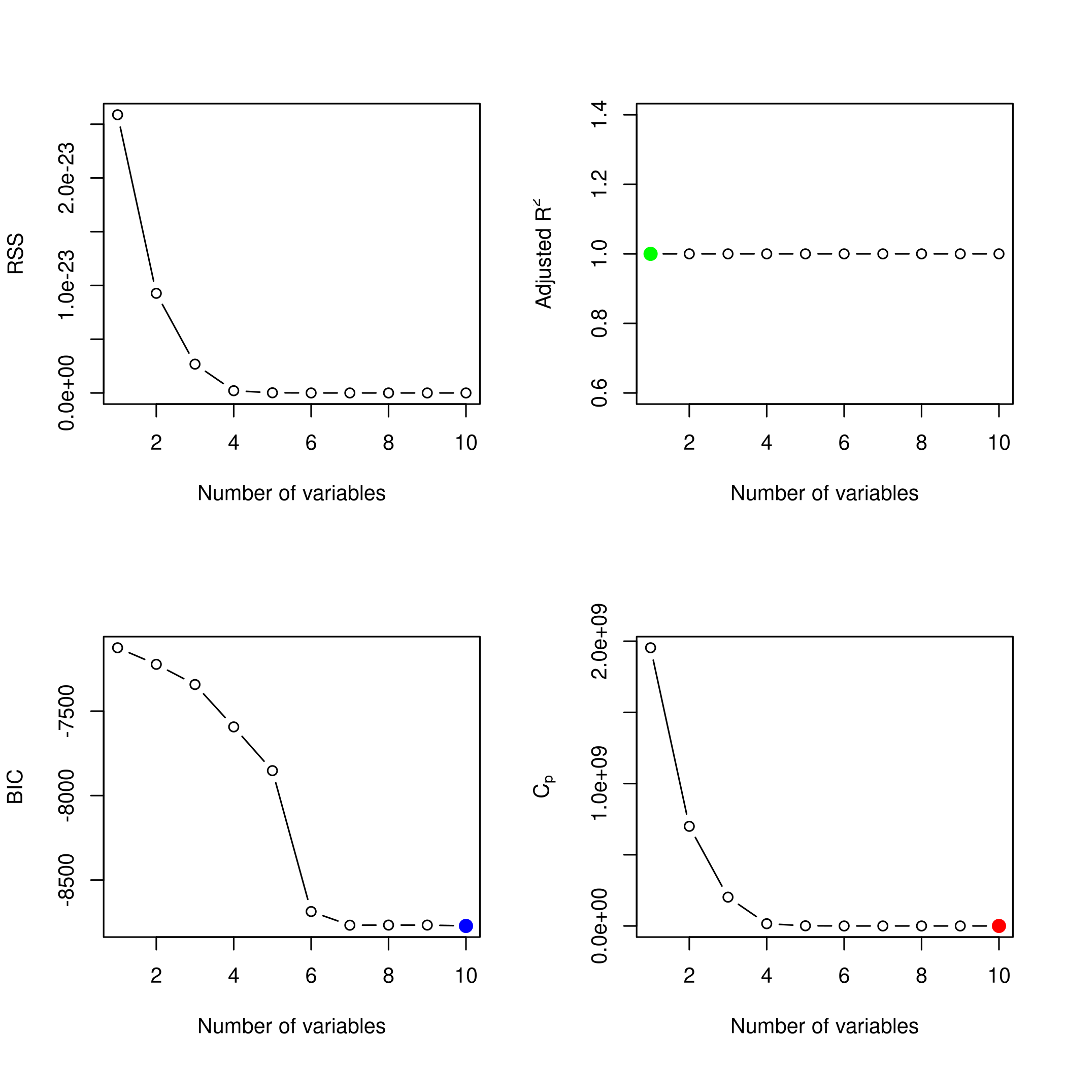
6 plot(leapObj$rss,xlab="Number of variables",ylab="RSS",type="b")
7 plot(leapObj$adjr2,xlab="Number of variables",ylab=TeX("Adjusted R^2"),type="b")
8 points(bar2,leapObj$adjr2[bar2],col="green",cex=2,pch=20)
9 plot(leapObj$bic,xlab="Number of variables",ylab=TeX("BIC"),type="b")
10 points(bbic,leapObj$bic[bbic],col="blue",cex=2,pch=20)
11 plot(leapObj$cp,xlab="Number of variables",ylab=TeX("C_p"),type="b")
12 points(bcp,leapObj$cp[bcp],col="red",cex=2,pch=20)
13}
1plotLEAP(forwardFit %>% summary)
Lets check the backward selection as well.
1modelX<-poly(x,10,raw=T)
2backwardFit<-regsubsets(y~modelX,data=df,nvmax=10,method="backward")
3backwardFit %>% summary %>% print
 1## Subset selection object
 2## Call: regsubsets.formula(y ~ modelX, data = df, nvmax = 10, method = "backward")
 3## 10 Variables  (and intercept)
 4##          Forced in Forced out
 5## modelX1      FALSE      FALSE
 6## modelX2      FALSE      FALSE
 7## modelX3      FALSE      FALSE
 8## modelX4      FALSE      FALSE
 9## modelX5      FALSE      FALSE
10## modelX6      FALSE      FALSE
11## modelX7      FALSE      FALSE
12## modelX8      FALSE      FALSE
13## modelX9      FALSE      FALSE
14## modelX10     FALSE      FALSE
15## 1 subsets of each size up to 10
16## Selection Algorithm: backward
17##           modelX1 modelX2 modelX3 modelX4 modelX5 modelX6 modelX7 modelX8
18## 1  ( 1 )  " "     " "     "*"     " "     " "     " "     " "     " "
19## 2  ( 1 )  "*"     " "     "*"     " "     " "     " "     " "     " "
20## 3  ( 1 )  "*"     " "     "*"     "*"     " "     " "     " "     " "
21## 4  ( 1 )  "*"     " "     "*"     "*"     " "     "*"     " "     " "
22## 5  ( 1 )  "*"     " "     "*"     "*"     " "     "*"     " "     "*"
23## 6  ( 1 )  "*"     " "     "*"     "*"     " "     "*"     " "     "*"
24## 7  ( 1 )  "*"     "*"     "*"     "*"     " "     "*"     " "     "*"
25## 8  ( 1 )  "*"     "*"     "*"     "*"     " "     "*"     "*"     "*"
26## 9  ( 1 )  "*"     "*"     "*"     "*"     " "     "*"     "*"     "*"
27## 10  ( 1 ) "*"     "*"     "*"     "*"     "*"     "*"     "*"     "*"
28##           modelX9 modelX10
29## 1  ( 1 )  " "     " "
30## 2  ( 1 )  " "     " "
31## 3  ( 1 )  " "     " "
32## 4  ( 1 )  " "     " "
33## 5  ( 1 )  " "     " "
34## 6  ( 1 )  " "     "*"
35## 7  ( 1 )  " "     "*"
36## 8  ( 1 )  " "     "*"
37## 9  ( 1 )  "*"     "*"
38## 10  ( 1 ) "*"     "*"
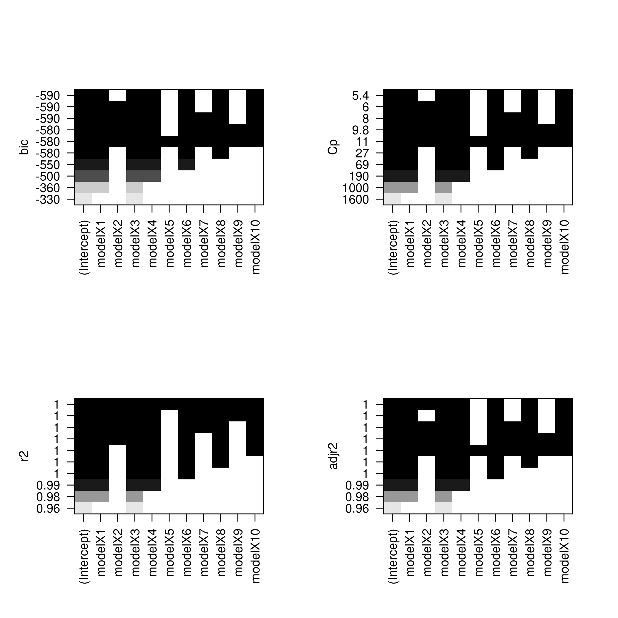
We might want to take a look at these.
1par(mfrow=c(2,2))
2plot(backwardFit)
3plot(backwardFit,scale='Cp')
4plot(backwardFit,scale='r2')
5plot(backwardFit,scale='adjr2')
1plotLEAP(backwardFit %>% summary)
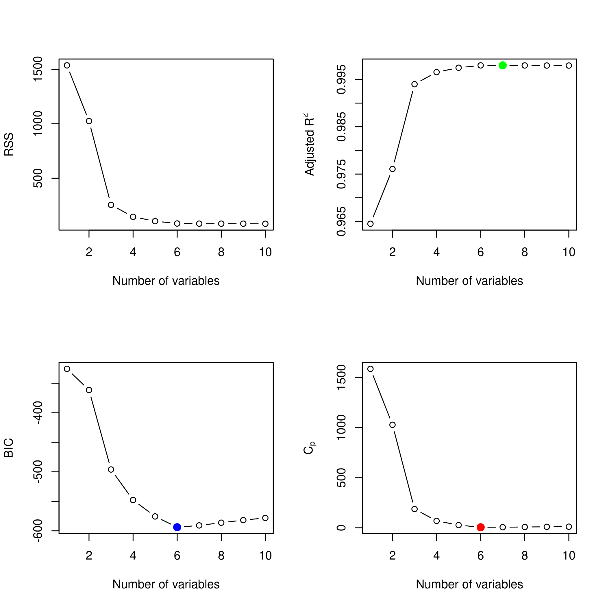
In spite of some slight variations, overall all methods converge to the
same best set of parameters, that of the third model.
e) LASSO and Cross Validation
For this, instead of using glmnet directly, we will use caret.
1df<-df %>% mutate(x2=x^2,x3=x^3,
2                  x4=x^4,x5=x^5,
3                  x6=x^6,x7=x^7,
4                  x8=x^8,x9=x^9,
5                  x10=x^10)
1lambda<-10^seq(-3, 3, length = 100)
2lassoCaret= train(y~.,data=df,method="glmnet",tuneGrid=expand.grid(alpha=1,lambda=lambda))
1## Warning in nominalTrainWorkflow(x = x, y = y, wts = weights, info = trainInfo, :
2## There were missing values in resampled performance measures.
1lassoCaret %>% print
1## glmnet
2##
3## 100 samples
4## 10 predictor
5##
6## No pre-processing
7## Resampling: Bootstrapped (25 reps)
8## Summary of sample sizes: 100, 100, 100, 100, 100, 100, ...
9## Resampling results across tuning parameters:
10##
11## lambda RMSE Rsquared MAE
12## 1.000000e-03 1.009696 0.9965632 0.8051425
13## 1.149757e-03 1.009696 0.9965632 0.8051425
14## 1.321941e-03 1.009696 0.9965632 0.8051425
15## 1.519911e-03 1.009696 0.9965632 0.8051425
16## 1.747528e-03 1.009696 0.9965632 0.8051425
17## 2.009233e-03 1.009696 0.9965632 0.8051425
18## 2.310130e-03 1.009696 0.9965632 0.8051425
19## 2.656088e-03 1.009696 0.9965632 0.8051425
20## 3.053856e-03 1.009696 0.9965632 0.8051425
21## 3.511192e-03 1.009696 0.9965632 0.8051425
22## 4.037017e-03 1.009696 0.9965632 0.8051425
23## 4.641589e-03 1.009696 0.9965632 0.8051425
24## 5.336699e-03 1.009696 0.9965632 0.8051425
25## 6.135907e-03 1.009696 0.9965632 0.8051425
26## 7.054802e-03 1.009696 0.9965632 0.8051425
27## 8.111308e-03 1.009696 0.9965632 0.8051425
28## 9.326033e-03 1.009696 0.9965632 0.8051425
29## 1.072267e-02 1.009696 0.9965632 0.8051425
30## 1.232847e-02 1.009696 0.9965632 0.8051425
31## 1.417474e-02 1.009696 0.9965632 0.8051425
32## 1.629751e-02 1.009696 0.9965632 0.8051425
33## 1.873817e-02 1.009696 0.9965632 0.8051425
34## 2.154435e-02 1.009696 0.9965632 0.8051425
35## 2.477076e-02 1.009696 0.9965632 0.8051425
36## 2.848036e-02 1.009696 0.9965632 0.8051425
37## 3.274549e-02 1.009696 0.9965632 0.8051425
38## 3.764936e-02 1.009696 0.9965632 0.8051425
39## 4.328761e-02 1.009696 0.9965632 0.8051425
40## 4.977024e-02 1.009696 0.9965632 0.8051425
41## 5.722368e-02 1.009696 0.9965632 0.8051425
42## 6.579332e-02 1.009696 0.9965632 0.8051425
43## 7.564633e-02 1.009637 0.9965632 0.8050666
44## 8.697490e-02 1.009216 0.9965637 0.8047862
45## 1.000000e-01 1.008901 0.9965636 0.8046468
46## 1.149757e-01 1.009470 0.9965616 0.8054790
47## 1.321941e-01 1.011206 0.9965561 0.8074253
48## 1.519911e-01 1.014475 0.9965476 0.8104930
49## 1.747528e-01 1.019202 0.9965383 0.8147296
50## 2.009233e-01 1.025943 0.9965259 0.8203974
51## 2.310130e-01 1.035374 0.9965094 0.8284187
52## 2.656088e-01 1.048294 0.9964878 0.8393282
53## 3.053856e-01 1.065717 0.9964592 0.8530952
54## 3.511192e-01 1.088903 0.9964215 0.8701072
55## 4.037017e-01 1.119433 0.9963715 0.8918217
56## 4.641589e-01 1.158919 0.9963053 0.9193677
57## 5.336699e-01 1.209841 0.9962136 0.9532842
58## 6.135907e-01 1.275467 0.9960778 0.9957151
59## 7.054802e-01 1.357247 0.9958966 1.0471169
60## 8.111308e-01 1.457886 0.9956561 1.1087362
61## 9.326033e-01 1.580743 0.9953362 1.1818188
62## 1.072267e+00 1.729330 0.9949070 1.2696235
63## 1.232847e+00 1.907599 0.9943306 1.3758463
64## 1.417474e+00 2.120178 0.9935518 1.5059031
65## 1.629751e+00 2.369642 0.9924954 1.6673393
66## 1.873817e+00 2.662906 0.9910539 1.8621728
67## 2.154435e+00 3.007271 0.9890638 2.0978907
68## 2.477076e+00 3.409377 0.9863097 2.3788439
69## 2.848036e+00 3.864727 0.9825900 2.7053428
70## 3.274549e+00 4.350785 0.9778541 3.0659309
71## 3.764936e+00 4.847045 0.9724311 3.4403210
72## 4.328761e+00 5.369017 0.9668240 3.8351441
73## 4.977024e+00 5.919492 0.9626812 4.2512694
74## 5.722368e+00 6.562134 0.9580843 4.7389049
75## 6.579332e+00 7.307112 0.9534537 5.2945905
76## 7.564633e+00 8.132296 0.9500300 5.8774541
77## 8.697490e+00 9.067321 0.9486589 6.4760997
78## 1.000000e+01 10.167822 0.9483195 7.1226569
79## 1.149757e+01 11.473284 0.9482975 7.8556639
80## 1.321941e+01 13.002703 0.9482975 8.6990451
81## 1.519911e+01 14.727852 0.9454119 9.6414650
82## 1.747528e+01 16.325210 0.9426796 10.5303097
83## 2.009233e+01 17.740599 0.9357286 11.3560865
84## 2.310130e+01 18.585795 0.9227167 11.8799668
85## 2.656088e+01 18.939596 0.9080584 12.1336575
86## 3.053856e+01 19.123568 0.9109065 12.2733471
87## 3.511192e+01 19.197966 NaN 12.3308613
88## 4.037017e+01 19.197966 NaN 12.3308613
89## 4.641589e+01 19.197966 NaN 12.3308613
90## 5.336699e+01 19.197966 NaN 12.3308613
91## 6.135907e+01 19.197966 NaN 12.3308613
92## 7.054802e+01 19.197966 NaN 12.3308613
93## 8.111308e+01 19.197966 NaN 12.3308613
94## 9.326033e+01 19.197966 NaN 12.3308613
95## 1.072267e+02 19.197966 NaN 12.3308613
96## 1.232847e+02 19.197966 NaN 12.3308613
97## 1.417474e+02 19.197966 NaN 12.3308613
98## 1.629751e+02 19.197966 NaN 12.3308613
99## 1.873817e+02 19.197966 NaN 12.3308613
100## 2.154435e+02 19.197966 NaN 12.3308613
101## 2.477076e+02 19.197966 NaN 12.3308613
102## 2.848036e+02 19.197966 NaN 12.3308613
103## 3.274549e+02 19.197966 NaN 12.3308613
104## 3.764936e+02 19.197966 NaN 12.3308613
105## 4.328761e+02 19.197966 NaN 12.3308613
106## 4.977024e+02 19.197966 NaN 12.3308613
107## 5.722368e+02 19.197966 NaN 12.3308613
108## 6.579332e+02 19.197966 NaN 12.3308613
109## 7.564633e+02 19.197966 NaN 12.3308613
110## 8.697490e+02 19.197966 NaN 12.3308613
111## 1.000000e+03 19.197966 NaN 12.3308613
112##
113## Tuning parameter 'alpha' was held constant at a value of 1
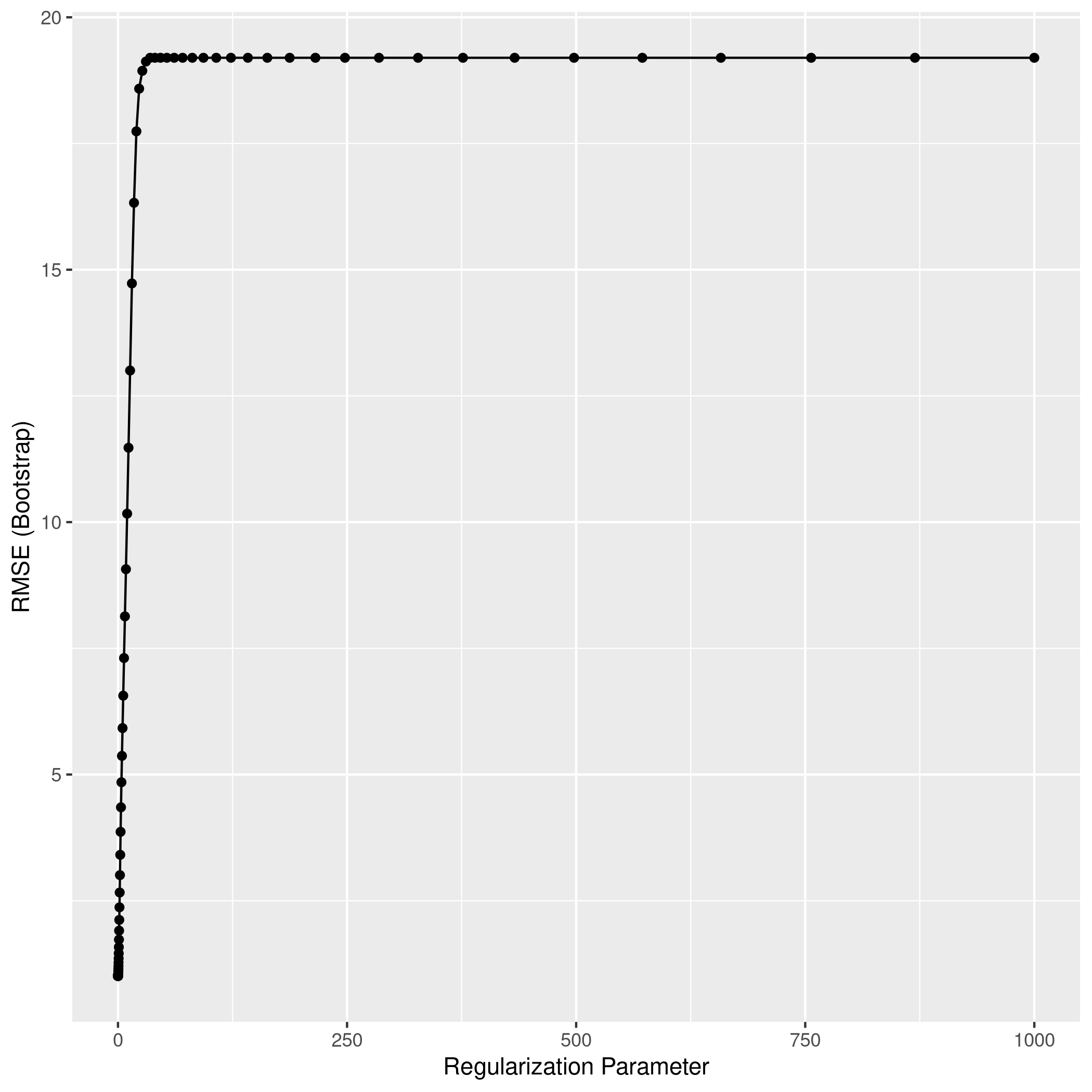
114## RMSE was used to select the optimal model using the smallest value.
115## The final values used for the model were alpha = 1 and lambda = 0.1.
1lassoCaret %>% ggplot
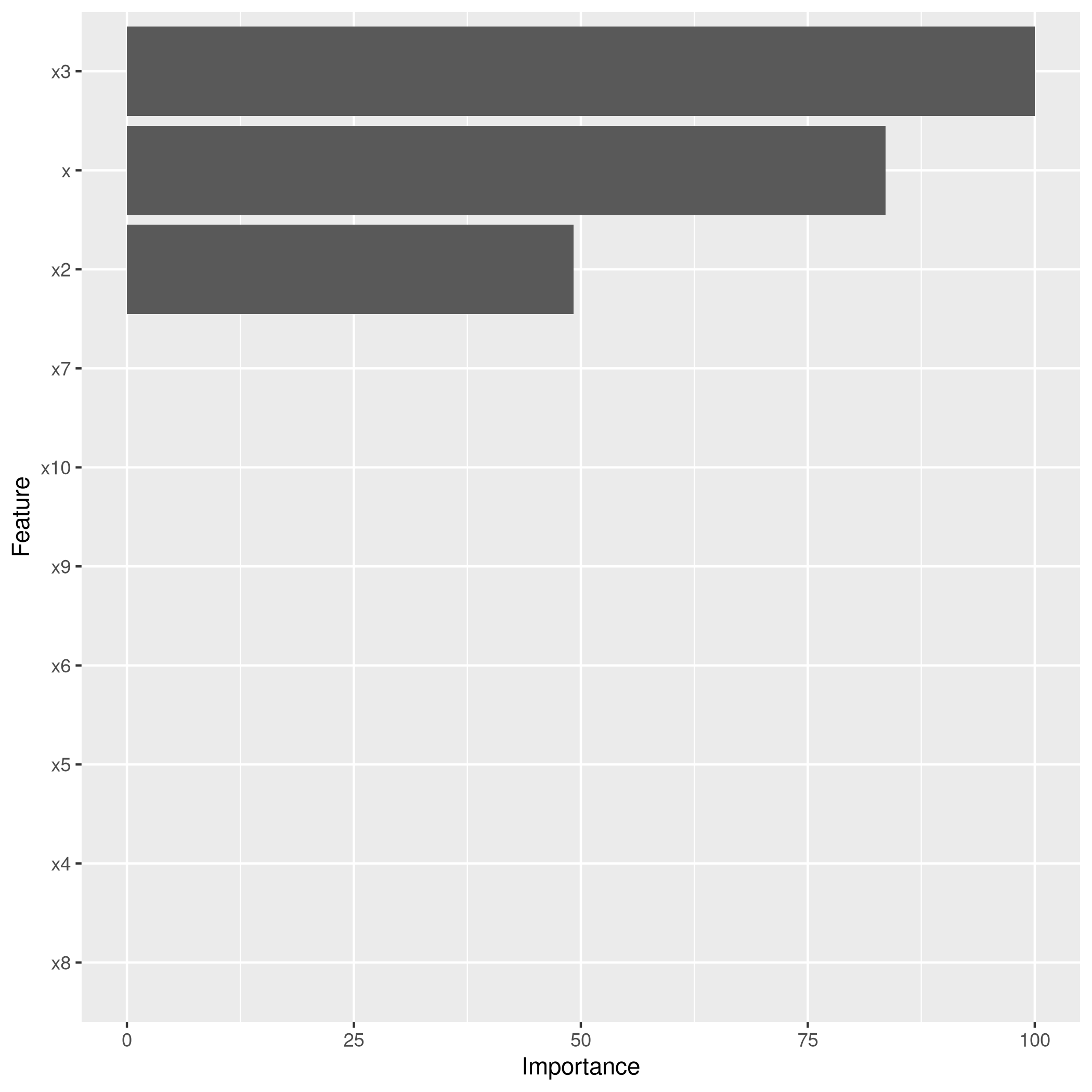
1lassoCaret %>% varImp %>% ggplot
1library(glmnet)
1## Loading required package: Matrix
1##
2## Attaching package: 'Matrix'
1## The following objects are masked from 'package:tidyr':
2##
3##     expand, pack, unpack
1## Loaded glmnet 3.0-2
1library(boot)
1##
2## Attaching package: 'boot'
1## The following object is masked from 'package:lattice':
2##
3##     melanoma
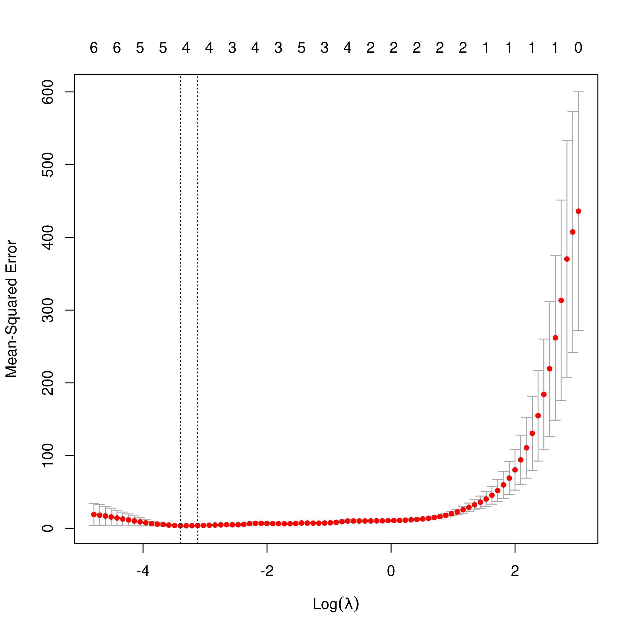
1lasso.mod <- cv.glmnet(as.matrix(df[-1]), y, alpha=1)
2lambda <- lasso.mod$lambda.min
3plot(lasso.mod)
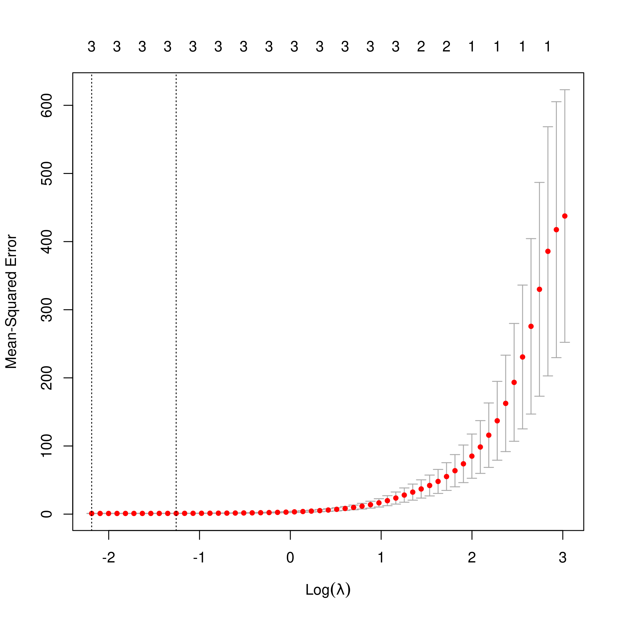
1predict(lasso.mod, s=lambda, type="coefficients")
 1## 11 x 1 sparse Matrix of class "dgCMatrix"
 2##                     1
 3## (Intercept) 42.975240
 4## x            5.005023
 5## x2           2.947540
 6## x3           5.989105
 7## x4           .
 8## x5           .
 9## x6           .
10## x7           .
11## x8           .
12## x9           .
13## x10          .
Clearly, the only important variables are \(x\), \(x^2\) and \(x^3\).
f) New model
Our new model requires a newly expanded set of betas as well.
1y2<-beta[1]+23*x^7+noise
1modelX<-poly(x,10,raw=T)
2newDF<-data.frame(x=as.matrix(modelX),y=y2)
3newSub<-regsubsets(y2~.,data=newDF,nvmax=10)
4newSub %>% summary
 1## Subset selection object
 2## Call: regsubsets.formula(y2 ~ ., data = newDF, nvmax = 10)
 3## 11 Variables  (and intercept)
 4##      Forced in Forced out
 5## x.1      FALSE      FALSE
 6## x.2      FALSE      FALSE
 7## x.3      FALSE      FALSE
 8## x.4      FALSE      FALSE
 9## x.5      FALSE      FALSE
10## x.6      FALSE      FALSE
11## x.7      FALSE      FALSE
12## x.8      FALSE      FALSE
13## x.9      FALSE      FALSE
14## x.10     FALSE      FALSE
15## y        FALSE      FALSE
16## 1 subsets of each size up to 10
17## Selection Algorithm: exhaustive
18##           x.1 x.2 x.3 x.4 x.5 x.6 x.7 x.8 x.9 x.10 y
19## 1  ( 1 )  " " " " " " " " " " " " " " " " " " " "  "*"
20## 2  ( 1 )  " " " " " " " " "*" " " " " " " " " " "  "*"
21## 3  ( 1 )  "*" "*" " " " " " " " " " " " " " " " "  "*"
22## 4  ( 1 )  "*" "*" "*" " " " " " " " " " " " " " "  "*"
23## 5  ( 1 )  "*" "*" "*" " " " " " " " " " " " " "*"  "*"
24## 6  ( 1 )  "*" "*" "*" "*" "*" " " " " " " " " " "  "*"
25## 7  ( 1 )  "*" "*" "*" "*" "*" " " "*" " " " " " "  "*"
26## 8  ( 1 )  "*" "*" "*" "*" "*" "*" "*" " " " " " "  "*"
27## 9  ( 1 )  "*" "*" "*" "*" "*" "*" "*" " " "*" " "  "*"
28## 10  ( 1 ) "*" "*" "*" "*" "*" "*" "*" "*" " " "*"  "*"
1plotLEAP(newSub %>% summary)
Or in its more native look,
1par(mfrow=c(2,2))
2plot(newSub)
3plot(newSub,scale='Cp')
4plot(newSub,scale='r2')
5plot(newSub,scale='adjr2')
1library(glmnet)
2library(boot)
3lasso.mod2 <- cv.glmnet(as.matrix(newDF[-1]), y, alpha=1)
4lambda2 <- lasso.mod2$lambda.min
5plot(lasso.mod2)
1predict(lasso.mod2, s=lambda, type="coefficients")
 1## 11 x 1 sparse Matrix of class "dgCMatrix"
 2##                       1
 3## (Intercept) 42.67982691
 4## x.2          3.22521396
 5## x.3          8.56699146
 6## x.4          .
 7## x.5         -0.10229572
 8## x.6          .
 9## x.7         -0.03184905
10## x.8          .
11## x.9          .
12## x.10         .
13## y            .
1lambda<-10^seq(-3, 3, length = 100)
2lassocaret2= train(y~.,data=newDF,method="glmnet",tuneGrid=expand.grid(alpha=1,lambda=lambda))
1## Warning in nominalTrainWorkflow(x = x, y = y, wts = weights, info = trainInfo, :
2## There were missing values in resampled performance measures.
1lassocaret2 %>% print
  1## glmnet
  2##
  3## 100 samples
  4##  10 predictor
  5##
  6## No pre-processing
  7## Resampling: Bootstrapped (25 reps)
  8## Summary of sample sizes: 100, 100, 100, 100, 100, 100, ...
  9## Resampling results across tuning parameters:
 10##
 11##   lambda        RMSE        Rsquared   MAE
 12##   1.000000e-03    40.03231  0.9999955   14.48774
 13##   1.149757e-03    40.03231  0.9999955   14.48774
 14##   1.321941e-03    40.03231  0.9999955   14.48774
 15##   1.519911e-03    40.03231  0.9999955   14.48774
 16##   1.747528e-03    40.03231  0.9999955   14.48774
 17##   2.009233e-03    40.03231  0.9999955   14.48774
 18##   2.310130e-03    40.03231  0.9999955   14.48774
 19##   2.656088e-03    40.03231  0.9999955   14.48774
 20##   3.053856e-03    40.03231  0.9999955   14.48774
 21##   3.511192e-03    40.03231  0.9999955   14.48774
 22##   4.037017e-03    40.03231  0.9999955   14.48774
 23##   4.641589e-03    40.03231  0.9999955   14.48774
 24##   5.336699e-03    40.03231  0.9999955   14.48774
 25##   6.135907e-03    40.03231  0.9999955   14.48774
 26##   7.054802e-03    40.03231  0.9999955   14.48774
 27##   8.111308e-03    40.03231  0.9999955   14.48774
 28##   9.326033e-03    40.03231  0.9999955   14.48774
 29##   1.072267e-02    40.03231  0.9999955   14.48774
 30##   1.232847e-02    40.03231  0.9999955   14.48774
 31##   1.417474e-02    40.03231  0.9999955   14.48774
 32##   1.629751e-02    40.03231  0.9999955   14.48774
 33##   1.873817e-02    40.03231  0.9999955   14.48774
 34##   2.154435e-02    40.03231  0.9999955   14.48774
 35##   2.477076e-02    40.03231  0.9999955   14.48774
 36##   2.848036e-02    40.03231  0.9999955   14.48774
 37##   3.274549e-02    40.03231  0.9999955   14.48774
 38##   3.764936e-02    40.03231  0.9999955   14.48774
 39##   4.328761e-02    40.03231  0.9999955   14.48774
 40##   4.977024e-02    40.03231  0.9999955   14.48774
 41##   5.722368e-02    40.03231  0.9999955   14.48774
 42##   6.579332e-02    40.03231  0.9999955   14.48774
 43##   7.564633e-02    40.03231  0.9999955   14.48774
 44##   8.697490e-02    40.03231  0.9999955   14.48774
 45##   1.000000e-01    40.03231  0.9999955   14.48774
 46##   1.149757e-01    40.03231  0.9999955   14.48774
 47##   1.321941e-01    40.03231  0.9999955   14.48774
 48##   1.519911e-01    40.03231  0.9999955   14.48774
 49##   1.747528e-01    40.03231  0.9999955   14.48774
 50##   2.009233e-01    40.03231  0.9999955   14.48774
 51##   2.310130e-01    40.03231  0.9999955   14.48774
 52##   2.656088e-01    40.03231  0.9999955   14.48774
 53##   3.053856e-01    40.03231  0.9999955   14.48774
 54##   3.511192e-01    40.03231  0.9999955   14.48774
 55##   4.037017e-01    40.03231  0.9999955   14.48774
 56##   4.641589e-01    40.03231  0.9999955   14.48774
 57##   5.336699e-01    40.03231  0.9999955   14.48774
 58##   6.135907e-01    40.03231  0.9999955   14.48774
 59##   7.054802e-01    40.03231  0.9999955   14.48774
 60##   8.111308e-01    40.03231  0.9999955   14.48774
 61##   9.326033e-01    40.03231  0.9999955   14.48774
 62##   1.072267e+00    40.03231  0.9999955   14.48774
 63##   1.232847e+00    40.03231  0.9999955   14.48774
 64##   1.417474e+00    40.03231  0.9999955   14.48774
 65##   1.629751e+00    40.03231  0.9999955   14.48774
 66##   1.873817e+00    40.03231  0.9999955   14.48774
 67##   2.154435e+00    40.03231  0.9999955   14.48774
 68##   2.477076e+00    40.03231  0.9999955   14.48774
 69##   2.848036e+00    40.03231  0.9999955   14.48774
 70##   3.274549e+00    40.03231  0.9999955   14.48774
 71##   3.764936e+00    40.03231  0.9999955   14.48774
 72##   4.328761e+00    40.03231  0.9999955   14.48774
 73##   4.977024e+00    40.03231  0.9999955   14.48774
 74##   5.722368e+00    40.03231  0.9999955   14.48774
 75##   6.579332e+00    40.03231  0.9999955   14.48774
 76##   7.564633e+00    40.43005  0.9999955   14.59881
 77##   8.697490e+00    41.25214  0.9999955   14.81913
 78##   1.000000e+01    42.30446  0.9999955   15.09937
 79##   1.149757e+01    43.59429  0.9999955   15.44307
 80##   1.321941e+01    45.43633  0.9999955   15.93255
 81##   1.519911e+01    47.55425  0.9999955   16.49605
 82##   1.747528e+01    49.98935  0.9999955   17.14447
 83##   2.009233e+01    52.90533  0.9999955   17.91650
 84##   2.310130e+01    57.57589  0.9999955   19.10125
 85##   2.656088e+01    63.25484  0.9999955   20.53147
 86##   3.053856e+01    70.51580  0.9999955   22.36400
 87##   3.511192e+01    78.93391  0.9999955   24.49105
 88##   4.037017e+01    88.61274  0.9999955   26.93830
 89##   4.641589e+01    99.97831  0.9999955   29.83601
 90##   5.336699e+01   113.48225  0.9999955   33.39320
 91##   6.135907e+01   129.17536  0.9999955   37.58303
 92##   7.054802e+01   147.76452  0.9999957   42.74333
 93##   8.111308e+01   169.60027  0.9999961   48.98043
 94##   9.326033e+01   194.94266  0.9999965   56.29001
 95##   1.072267e+02   224.07631  0.9999969   64.70026
 96##   1.232847e+02   257.56092  0.9999971   74.36989
 97##   1.417474e+02   296.13382  0.9999971   85.51504
 98##   1.629751e+02   340.49129  0.9999971   98.33212
 99##   1.873817e+02   391.49185  0.9999971  113.06864
100##   2.154435e+02   450.13031  0.9999971  130.01206
101##   2.477076e+02   509.28329  0.9999970  147.15405
102##   2.848036e+02   564.17558  0.9999969  163.34475
103##   3.274549e+02   618.84080  0.9999969  179.85589
104##   3.764936e+02   681.69265  0.9999969  198.83969
105##   4.328761e+02   741.14452  0.9999967  217.28049
106##   4.977024e+02   807.25385  0.9999967  237.88938
107##   5.722368e+02   883.26360  0.9999967  261.58461
108##   6.579332e+02   970.65640  0.9999967  288.82836
109##   7.564633e+02  1037.84801  0.9999960  312.54099
110##   8.697490e+02  1088.92551  0.9999960  334.04769
111##   1.000000e+03  1131.46176  0.9999955  354.62317
112##
113## Tuning parameter 'alpha' was held constant at a value of 1
114## RMSE was used to select the optimal model using the smallest value.
115## The final values used for the model were alpha = 1 and lambda = 6.579332.
1lassocaret2 %>% ggplot
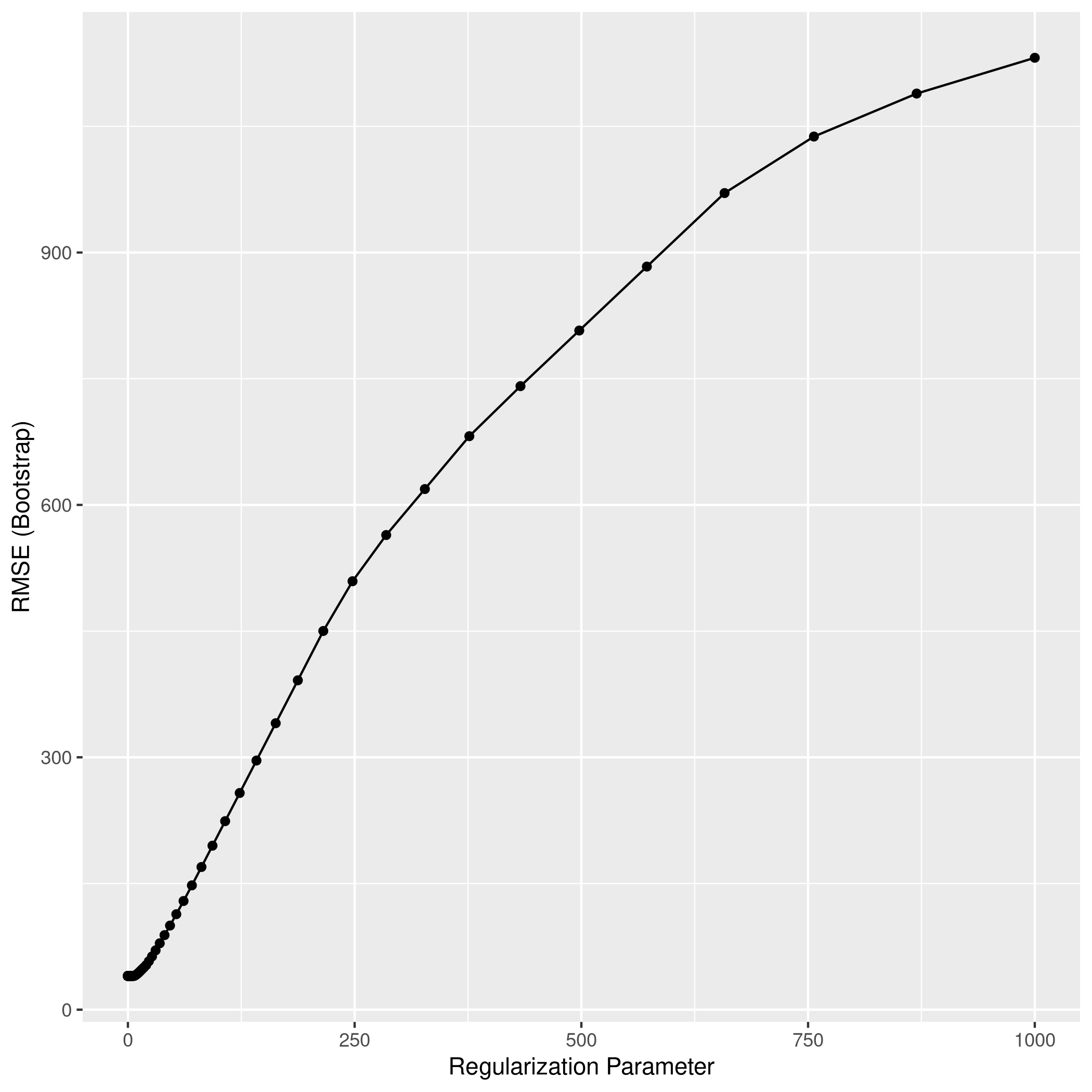
1lassocaret2 %>% varImp %>% ggplot
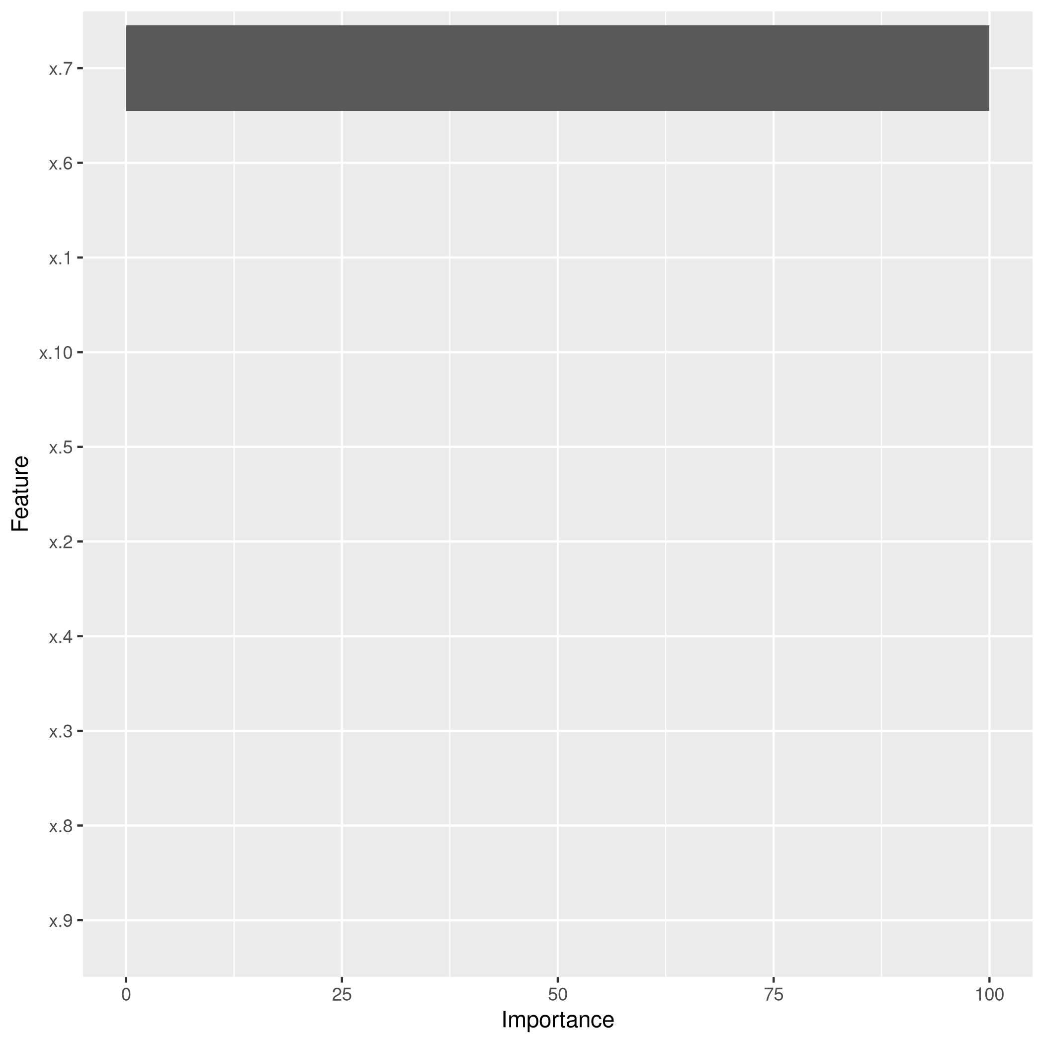
Clearly, the LASSO model has correctly reduced the model down to the correct single variable form, though best subset seems to suggest using more predictors, their coefficients are low enough to recognize that they are noise.
Question 6.9 - Page 263
In this exercise, we will predict the number of applications received
using the other variables in the College data set.
(a) Split the data set into a training set and a test set.
(b) Fit a linear model using least squares on the training set, and report the test error obtained.
(c) Fit a ridge regression model on the training set, with \(\lambda\) chosen by cross-validation. Report the test error obtained.
(d) Fit a lasso model on the training set, with \(\lambda\) chosen by crossvalidation. Report the test error obtained, along with the number of non-zero coefficient estimates.
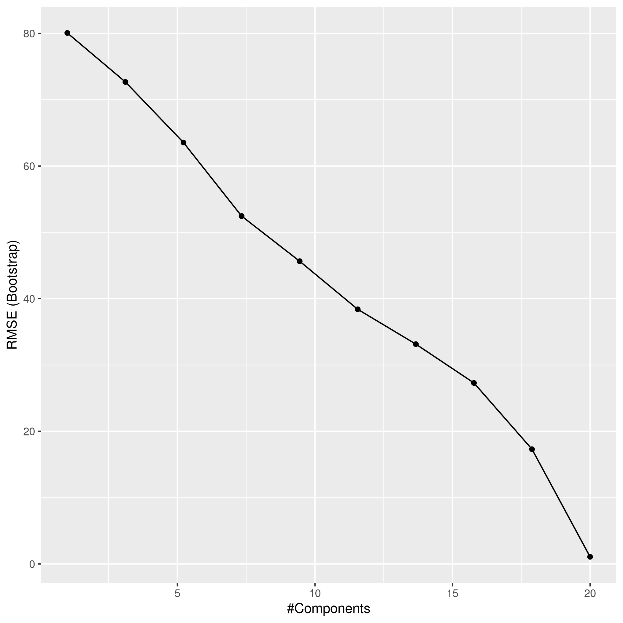
(e) Fit a PCR model on the training set, with \(M\) chosen by crossvalidation. Report the test error obtained, along with the value of \(M\) selected by cross-validation.
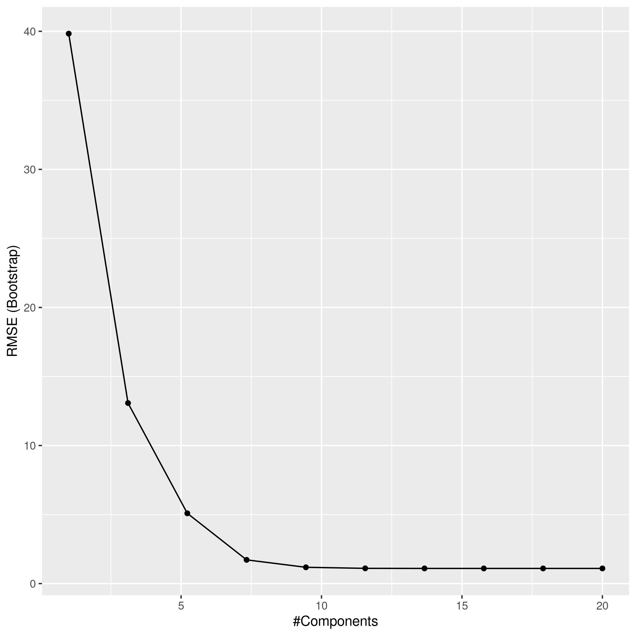
(f) Fit a PLS model on the training set, with M chosen by crossvalidation. Report the test error obtained, along with the value of M selected by cross-validation.
(g) Comment on the results obtained. How accurately can we predict the number of college applications received? Is there much difference among the test errors resulting from these five approaches?
Answer
We will use the caret package, since at the moment, mlr3 does not
have learners for PCR and PLS.
1colDat<-ISLR::College
2colDat %>% summary %>% print
 1##  Private        Apps           Accept          Enroll       Top10perc
 2##  No :212   Min.   :   81   Min.   :   72   Min.   :  35   Min.   : 1.00
 3##  Yes:565   1st Qu.:  776   1st Qu.:  604   1st Qu.: 242   1st Qu.:15.00
 4##            Median : 1558   Median : 1110   Median : 434   Median :23.00
 5##            Mean   : 3002   Mean   : 2019   Mean   : 780   Mean   :27.56
 6##            3rd Qu.: 3624   3rd Qu.: 2424   3rd Qu.: 902   3rd Qu.:35.00
 7##            Max.   :48094   Max.   :26330   Max.   :6392   Max.   :96.00
 8##    Top25perc      F.Undergrad     P.Undergrad         Outstate
 9##  Min.   :  9.0   Min.   :  139   Min.   :    1.0   Min.   : 2340
10##  1st Qu.: 41.0   1st Qu.:  992   1st Qu.:   95.0   1st Qu.: 7320
11##  Median : 54.0   Median : 1707   Median :  353.0   Median : 9990
12##  Mean   : 55.8   Mean   : 3700   Mean   :  855.3   Mean   :10441
13##  3rd Qu.: 69.0   3rd Qu.: 4005   3rd Qu.:  967.0   3rd Qu.:12925
14##  Max.   :100.0   Max.   :31643   Max.   :21836.0   Max.   :21700
15##    Room.Board       Books           Personal         PhD
16##  Min.   :1780   Min.   :  96.0   Min.   : 250   Min.   :  8.00
17##  1st Qu.:3597   1st Qu.: 470.0   1st Qu.: 850   1st Qu.: 62.00
18##  Median :4200   Median : 500.0   Median :1200   Median : 75.00
19##  Mean   :4358   Mean   : 549.4   Mean   :1341   Mean   : 72.66
20##  3rd Qu.:5050   3rd Qu.: 600.0   3rd Qu.:1700   3rd Qu.: 85.00
21##  Max.   :8124   Max.   :2340.0   Max.   :6800   Max.   :103.00
22##     Terminal       S.F.Ratio      perc.alumni        Expend
23##  Min.   : 24.0   Min.   : 2.50   Min.   : 0.00   Min.   : 3186
24##  1st Qu.: 71.0   1st Qu.:11.50   1st Qu.:13.00   1st Qu.: 6751
25##  Median : 82.0   Median :13.60   Median :21.00   Median : 8377
26##  Mean   : 79.7   Mean   :14.09   Mean   :22.74   Mean   : 9660
27##  3rd Qu.: 92.0   3rd Qu.:16.50   3rd Qu.:31.00   3rd Qu.:10830
28##  Max.   :100.0   Max.   :39.80   Max.   :64.00   Max.   :56233
29##    Grad.Rate
30##  Min.   : 10.00
31##  1st Qu.: 53.00
32##  Median : 65.00
33##  Mean   : 65.46
34##  3rd Qu.: 78.00
35##  Max.   :118.00
1colDat %>% str %>% print
 1## 'data.frame':    777 obs. of  18 variables:
 2##  $ Private    : Factor w/ 2 levels "No","Yes": 2 2 2 2 2 2 2 2 2 2 ...
 3##  $ Apps       : num  1660 2186 1428 417 193 ...
 4##  $ Accept     : num  1232 1924 1097 349 146 ...
 5##  $ Enroll     : num  721 512 336 137 55 158 103 489 227 172 ...
 6##  $ Top10perc  : num  23 16 22 60 16 38 17 37 30 21 ...
 7##  $ Top25perc  : num  52 29 50 89 44 62 45 68 63 44 ...
 8##  $ F.Undergrad: num  2885 2683 1036 510 249 ...
 9##  $ P.Undergrad: num  537 1227 99 63 869 ...
10##  $ Outstate   : num  7440 12280 11250 12960 7560 ...
11##  $ Room.Board : num  3300 6450 3750 5450 4120 ...
12##  $ Books      : num  450 750 400 450 800 500 500 450 300 660 ...
13##  $ Personal   : num  2200 1500 1165 875 1500 ...
14##  $ PhD        : num  70 29 53 92 76 67 90 89 79 40 ...
15##  $ Terminal   : num  78 30 66 97 72 73 93 100 84 41 ...
16##  $ S.F.Ratio  : num  18.1 12.2 12.9 7.7 11.9 9.4 11.5 13.7 11.3 11.5 ...
17##  $ perc.alumni: num  12 16 30 37 2 11 26 37 23 15 ...
18##  $ Expend     : num  7041 10527 8735 19016 10922 ...
19##  $ Grad.Rate  : num  60 56 54 59 15 55 63 73 80 52 ...
20## NULL
1colDat %>% sapply(unique) %>% sapply(length) %>% print
1##     Private        Apps      Accept      Enroll   Top10perc   Top25perc
2##           2         711         693         581          82          89
3## F.Undergrad P.Undergrad    Outstate  Room.Board       Books    Personal
4##         714         566         640         553         122         294
5##         PhD    Terminal   S.F.Ratio perc.alumni      Expend   Grad.Rate
6##          78          65         173          61         744          81
Clearly, there are no psuedo-factors which might have been converted at this stage.
a) Train-Test split
1train_ind<-createDataPartition(colDat$Apps,p=0.8,times=1,list=FALSE)
2train_set<-colDat[train_ind,]
3test_set<-colDat[-train_ind,]
b) Linear least squares
1linCol<-train(Apps~.,data=train_set,method="lm")
2linCol %>% summary
 1##
 2## Call:
 3## lm(formula = .outcome ~ ., data = dat)
 4##
 5## Residuals:
 6##     Min      1Q  Median      3Q     Max
 7## -5145.6  -414.8   -20.3   340.5  7526.8
 8##
 9## Coefficients:
10##               Estimate Std. Error t value Pr(>|t|)
11## (Intercept) -2.918e+02  4.506e+02  -0.648 0.517486
12## PrivateYes  -5.351e+02  1.532e+02  -3.494 0.000511 ***
13## Accept       1.617e+00  4.258e-02  37.983  < 2e-16 ***
14## Enroll      -1.012e+00  1.959e-01  -5.165 3.26e-07 ***
15## Top10perc    5.379e+01  6.221e+00   8.647  < 2e-16 ***
16## Top25perc   -1.632e+01  5.046e+00  -3.235 0.001282 **
17## F.Undergrad  6.836e-02  3.457e-02   1.978 0.048410 *
18## P.Undergrad  7.929e-02  3.367e-02   2.355 0.018854 *
19## Outstate    -7.303e-02  2.098e-02  -3.481 0.000536 ***
20## Room.Board   1.695e-01  5.367e-02   3.159 0.001663 **
21## Books        9.998e-02  2.578e-01   0.388 0.698328
22## Personal    -3.145e-03  6.880e-02  -0.046 0.963553
23## PhD         -8.926e+00  5.041e+00  -1.771 0.077112 .
24## Terminal    -2.298e+00  5.608e+00  -0.410 0.682152
25## S.F.Ratio    6.038e+00  1.420e+01   0.425 0.670757
26## perc.alumni -5.085e-01  4.560e+00  -0.112 0.911249
27## Expend       4.668e-02  1.332e-02   3.505 0.000490 ***
28## Grad.Rate    9.042e+00  3.379e+00   2.676 0.007653 **
29## ---
30## Signif. codes:  0 '***' 0.001 '**' 0.01 '*' 0.05 '.' 0.1 ' ' 1
31##
32## Residual standard error: 1042 on 606 degrees of freedom
33## Multiple R-squared:  0.9332, Adjusted R-squared:  0.9313
34## F-statistic: 497.7 on 17 and 606 DF,  p-value: < 2.2e-16
1linPred<-predict(linCol,test_set)
2linPred %>% postResample(obs = test_set$Apps)
1##         RMSE     Rsquared          MAE
2## 1071.6360025    0.9017032  625.7827996
Do note that the metrics are calculated in a manner to ensure no negative values are obtained.
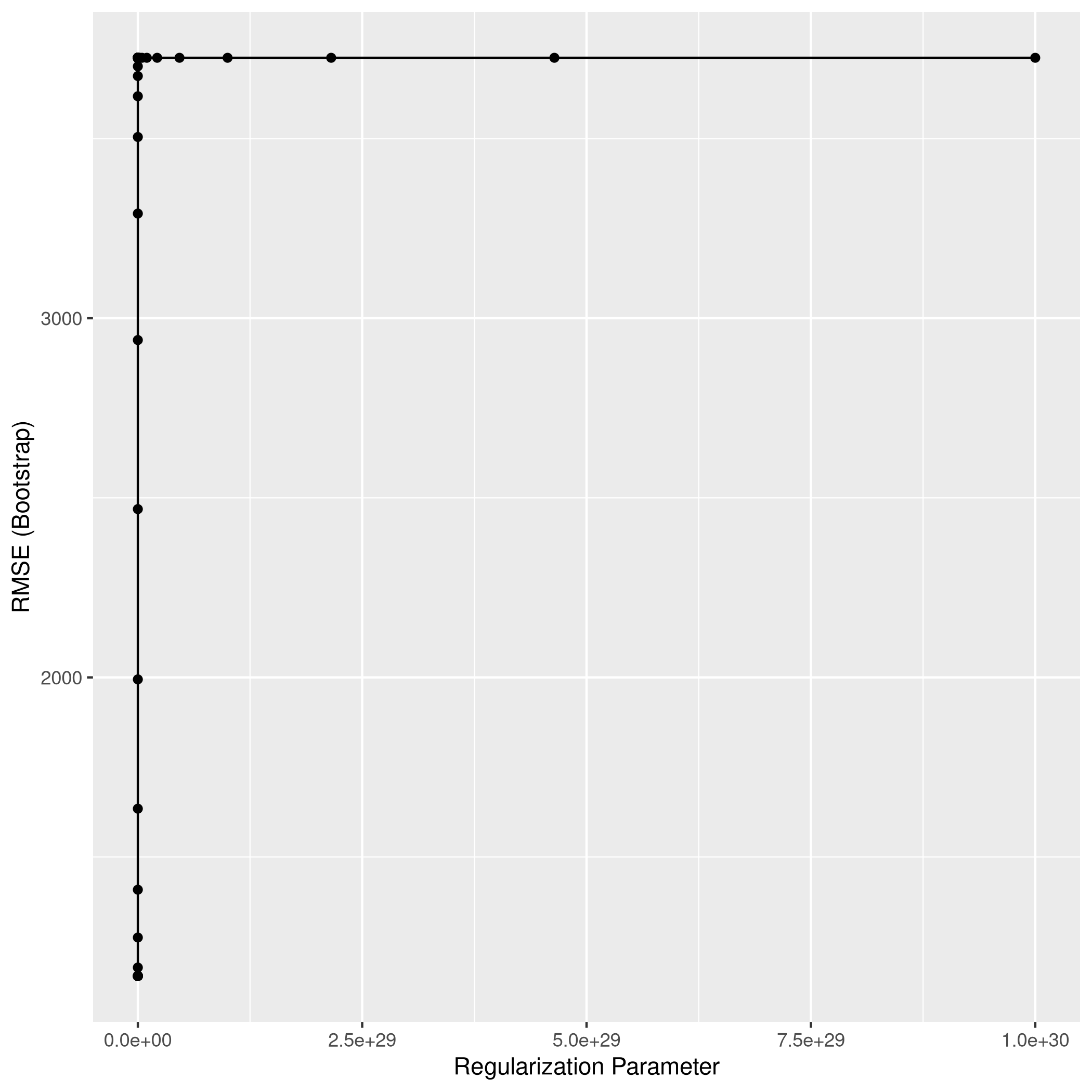
c) Ridge regression with CV for λ
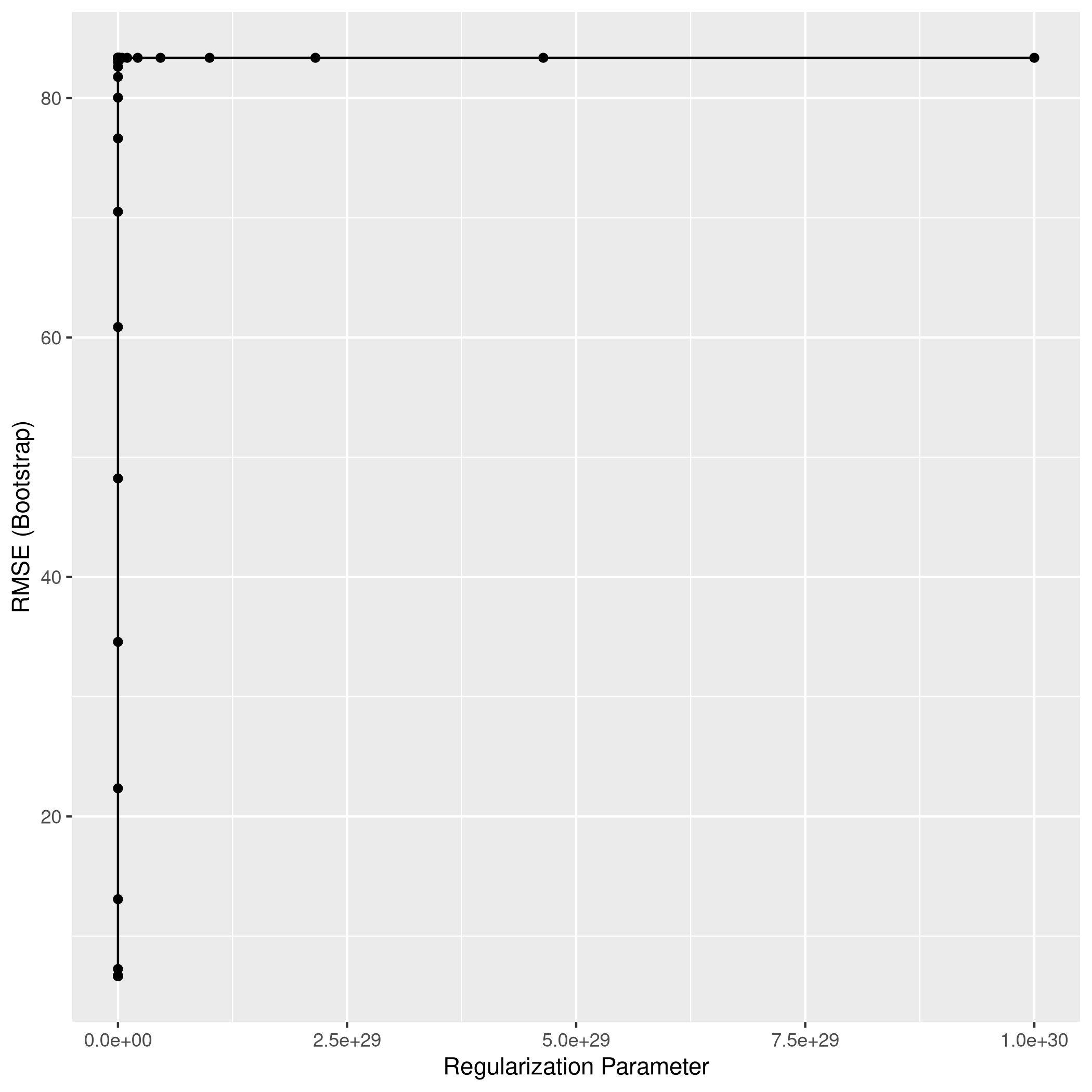
1L2Grid <- expand.grid(alpha=0,
2                          lambda=10^seq(from=-3,to=30,length=100))
1ridgCol<-train(Apps~.,data=train_set,method="glmnet",tuneGrid = L2Grid)
1## Warning in nominalTrainWorkflow(x = x, y = y, wts = weights, info = trainInfo, :
2## There were missing values in resampled performance measures.
1ridgCol %>% summary %>% print
 1##             Length Class      Mode
 2## a0           100   -none-     numeric
 3## beta        1700   dgCMatrix  S4
 4## df           100   -none-     numeric
 5## dim            2   -none-     numeric
 6## lambda       100   -none-     numeric
 7## dev.ratio    100   -none-     numeric
 8## nulldev        1   -none-     numeric
 9## npasses        1   -none-     numeric
10## jerr           1   -none-     numeric
11## offset         1   -none-     logical
12## call           5   -none-     call
13## nobs           1   -none-     numeric
14## lambdaOpt      1   -none-     numeric
15## xNames        17   -none-     character
16## problemType    1   -none-     character
17## tuneValue      2   data.frame list
18## obsLevels      1   -none-     logical
19## param          0   -none-     list
1coef(ridgCol$finalModel, ridgCol$bestTune$lambda) %>% print
 1## 18 x 1 sparse Matrix of class "dgCMatrix"
 2##                         1
 3## (Intercept) -1.407775e+03
 4## PrivateYes  -5.854245e+02
 5## Accept       1.042778e+00
 6## Enroll       3.511219e-01
 7## Top10perc    2.780211e+01
 8## Top25perc    2.883536e-02
 9## F.Undergrad  6.825141e-02
10## P.Undergrad  5.281320e-02
11## Outstate    -2.011504e-02
12## Room.Board   2.155224e-01
13## Books        1.517585e-01
14## Personal    -3.711406e-02
15## PhD         -4.453155e+00
16## Terminal    -3.783231e+00
17## S.F.Ratio    6.897360e+00
18## perc.alumni -9.301831e+00
19## Expend       5.601144e-02
20## Grad.Rate    1.259989e+01
1ggplot(ridgCol)
1ridgPred<-predict(ridgCol,test_set)
2ridgPred %>% postResample(obs = test_set$Apps)
1##         RMSE     Rsquared          MAE
2## 1047.7545250    0.9051726  644.4535063
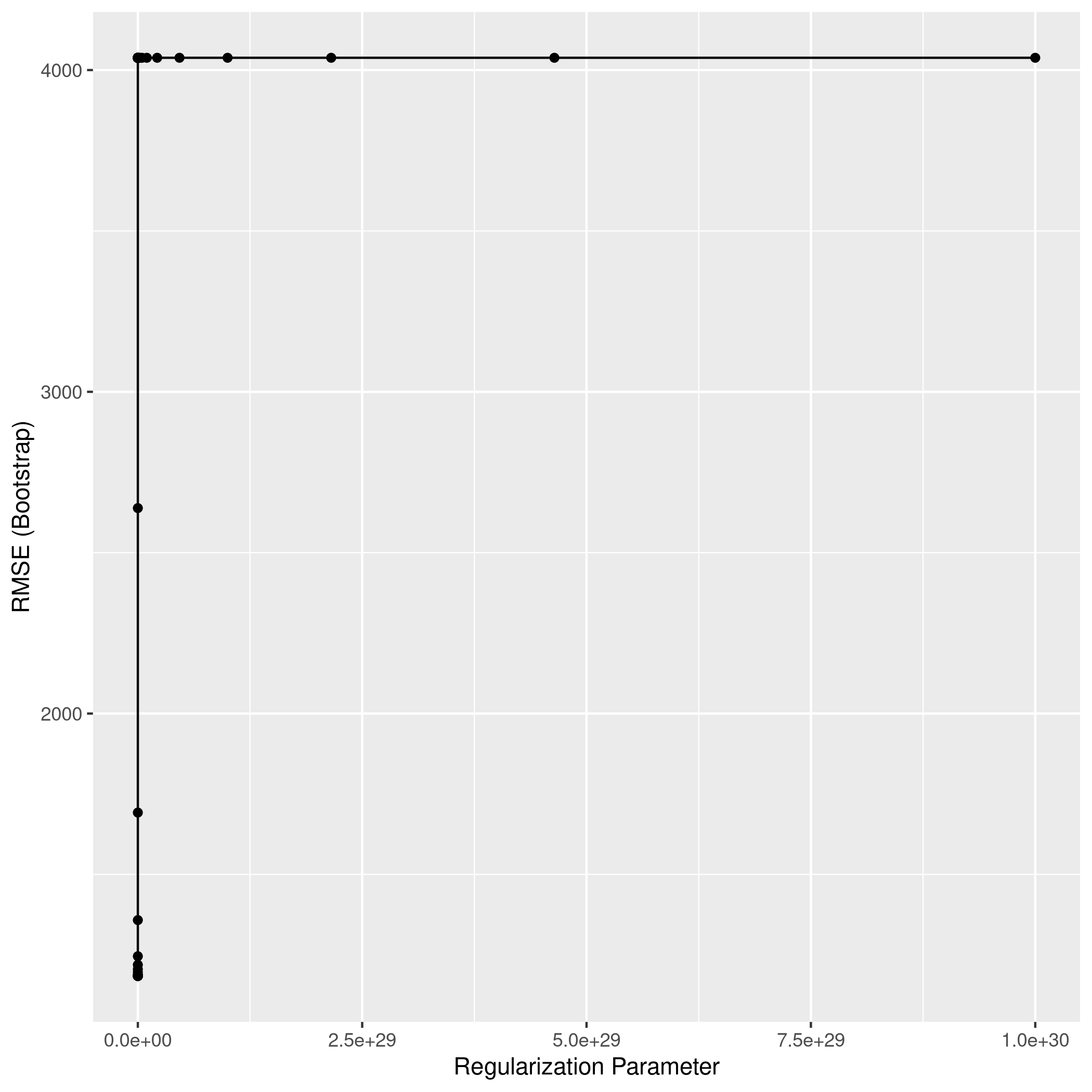
d) LASSO with CV for λ
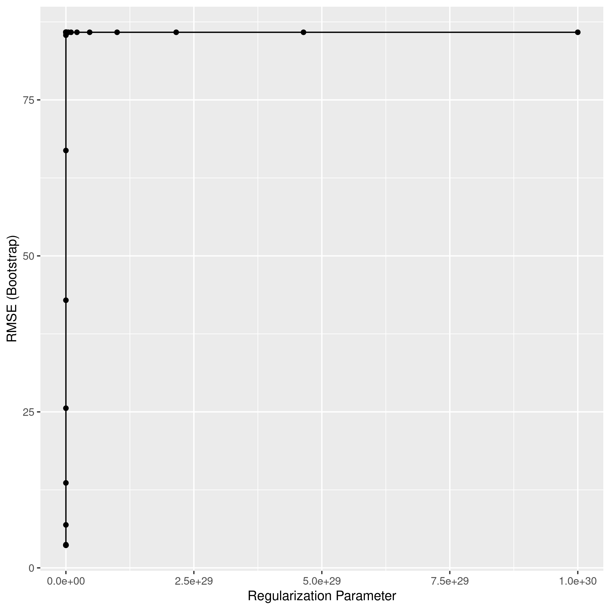
1L1Grid <- expand.grid(alpha=1, # for lasso
2                          lambda=10^seq(from=-3,to=30,length=100))
1lassoCol<-train(Apps~.,data=train_set,method="glmnet",tuneGrid = L1Grid)
1## Warning in nominalTrainWorkflow(x = x, y = y, wts = weights, info = trainInfo, :
2## There were missing values in resampled performance measures.
1lassoCol %>% summary %>% print
 1##             Length Class      Mode
 2## a0            81   -none-     numeric
 3## beta        1377   dgCMatrix  S4
 4## df            81   -none-     numeric
 5## dim            2   -none-     numeric
 6## lambda        81   -none-     numeric
 7## dev.ratio     81   -none-     numeric
 8## nulldev        1   -none-     numeric
 9## npasses        1   -none-     numeric
10## jerr           1   -none-     numeric
11## offset         1   -none-     logical
12## call           5   -none-     call
13## nobs           1   -none-     numeric
14## lambdaOpt      1   -none-     numeric
15## xNames        17   -none-     character
16## problemType    1   -none-     character
17## tuneValue      2   data.frame list
18## obsLevels      1   -none-     logical
19## param          0   -none-     list
1coef(lassoCol$finalModel, lassoCol$bestTune$lambda) %>% print
 1## 18 x 1 sparse Matrix of class "dgCMatrix"
 2##                         1
 3## (Intercept) -325.51554340
 4## PrivateYes  -532.28956305
 5## Accept         1.60370798
 6## Enroll        -0.90158328
 7## Top10perc     51.96610325
 8## Top25perc    -14.87886847
 9## F.Undergrad    0.05352324
10## P.Undergrad    0.07832395
11## Outstate      -0.07047302
12## Room.Board     0.16783269
13## Books          0.08836704
14## Personal       .
15## PhD           -8.67634519
16## Terminal      -2.18494018
17## S.F.Ratio      5.25050018
18## perc.alumni   -0.67848535
19## Expend         0.04597728
20## Grad.Rate      8.67569015
1ggplot(lassoCol)
1lassoPred<-predict(lassoCol,test_set)
2lassoPred %>% postResample(obs = test_set$Apps)
1##         RMSE     Rsquared          MAE
2## 1068.9834769    0.9021268  622.7029418
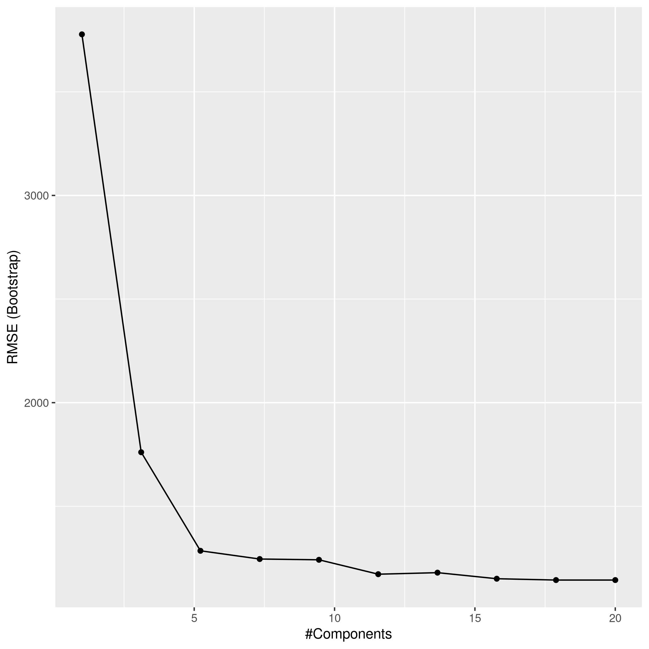
e) PCR with CV for M
1mGrid <- expand.grid(ncomp=seq(from=1,to=20,length=10))
1pcrCol<-train(Apps~.,data=train_set,method="pcr",tuneGrid = mGrid)
2pcrCol %>% summary %>% print
 1## Data:    X dimension: 624 17
 2##  Y dimension: 624 1
 3## Fit method: svdpc
 4## Number of components considered: 17
 5## TRAINING: % variance explained
 6##           1 comps  2 comps  3 comps  4 comps  5 comps  6 comps  7 comps
 7## X         48.2314    87.24    95.02    97.26    98.63    99.43    99.91
 8## .outcome   0.2419    76.54    77.88    80.19    91.27    91.34    91.34
 9##           8 comps  9 comps  10 comps  11 comps  12 comps  13 comps  14 comps
10## X           99.96   100.00    100.00    100.00    100.00    100.00    100.00
11## .outcome    91.65    91.66     92.26     92.65     92.66     92.67     92.76
12##           15 comps  16 comps  17 comps
13## X           100.00    100.00    100.00
14## .outcome     93.17     93.18     93.32
15## NULL
1ggplot(pcrCol)
1pcrPred<-predict(pcrCol,test_set)
2pcrPred %>% postResample(obs = test_set$Apps)
1##         RMSE     Rsquared          MAE
2## 1071.6360025    0.9017032  625.7827996
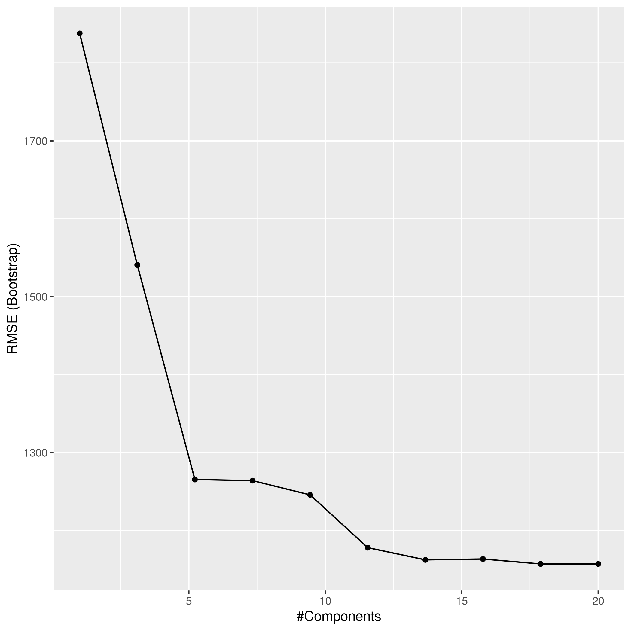
f) PLS with CV for M
1plsCol<-train(Apps~.,data=train_set,method="pls",tuneGrid = mGrid)
2plsCol %>% summary %>% print
 1## Data:    X dimension: 624 17
 2##  Y dimension: 624 1
 3## Fit method: oscorespls
 4## Number of components considered: 17
 5## TRAINING: % variance explained
 6##           1 comps  2 comps  3 comps  4 comps  5 comps  6 comps  7 comps
 7## X           39.02     56.4    91.83    96.61    98.62    99.22    99.49
 8## .outcome    78.04     84.1    86.88    91.09    91.38    91.49    91.66
 9##           8 comps  9 comps  10 comps  11 comps  12 comps  13 comps  14 comps
10## X           99.96    99.99    100.00    100.00    100.00    100.00    100.00
11## .outcome    91.68    91.85     92.64     92.87     93.16     93.18     93.18
12##           15 comps  16 comps  17 comps
13## X           100.00    100.00    100.00
14## .outcome     93.18     93.19     93.32
15## NULL
1ggplot(plsCol)
1plsPred<-predict(plsCol,test_set)
2plsPred %>% postResample(obs = test_set$Apps)
1##         RMSE     Rsquared          MAE
2## 1071.6360039    0.9017032  625.7827987
g) Comments and Comparison
1models <- list(ridge = ridgCol, lasso = lassoCol, pcr = pcrCol, pls=plsCol,linear=linCol)
2resamples(models) %>% summary
 1##
 2## Call:
 3## summary.resamples(object = .)
 4##
 5## Models: ridge, lasso, pcr, pls, linear
 6## Number of resamples: 25
 7##
 8## MAE
 9##            Min.  1st Qu.   Median     Mean  3rd Qu.     Max. NA's
10## ridge  536.9612 600.5398 623.2005 649.6713 707.4014 793.4972    0
11## lasso  573.8563 616.3883 671.9453 655.8858 691.7620 732.2155    0
12## pcr    576.1427 618.8694 650.0360 662.9040 714.8491 767.5535    0
13## pls    553.3999 607.9757 637.1985 638.6619 668.5120 735.4479    0
14## linear 556.5553 619.2395 654.1478 659.4635 686.7747 792.4912    0
15##
16## RMSE
17##            Min.   1st Qu.   Median     Mean  3rd Qu.     Max. NA's
18## ridge  882.2646  920.5934 1000.519 1168.603 1163.377 1939.541    0
19## lasso  801.9415  990.0724 1168.234 1184.329 1302.221 1584.712    0
20## pcr    828.1370  942.2678 1131.207 1144.071 1284.178 1544.078    0
21## pls    786.7989 1038.3265 1167.764 1157.026 1274.041 1461.434    0
22## linear 798.3771 1063.3690 1134.291 1135.977 1215.115 1403.576    0
23##
24## Rsquared
25##             Min.   1st Qu.    Median      Mean   3rd Qu.      Max. NA's
26## ridge  0.8735756 0.8962010 0.9185736 0.9136429 0.9306819 0.9474913    0
27## lasso  0.8851991 0.9132766 0.9217660 0.9191638 0.9284838 0.9398772    0
28## pcr    0.8658504 0.9080179 0.9235117 0.9146884 0.9281892 0.9471991    0
29## pls    0.8881249 0.9080786 0.9183968 0.9173632 0.9258994 0.9420894    0
30## linear 0.8840049 0.8986452 0.9222319 0.9160913 0.9296275 0.9492198    0
1resamples(models) %>% bwplot(scales="free")
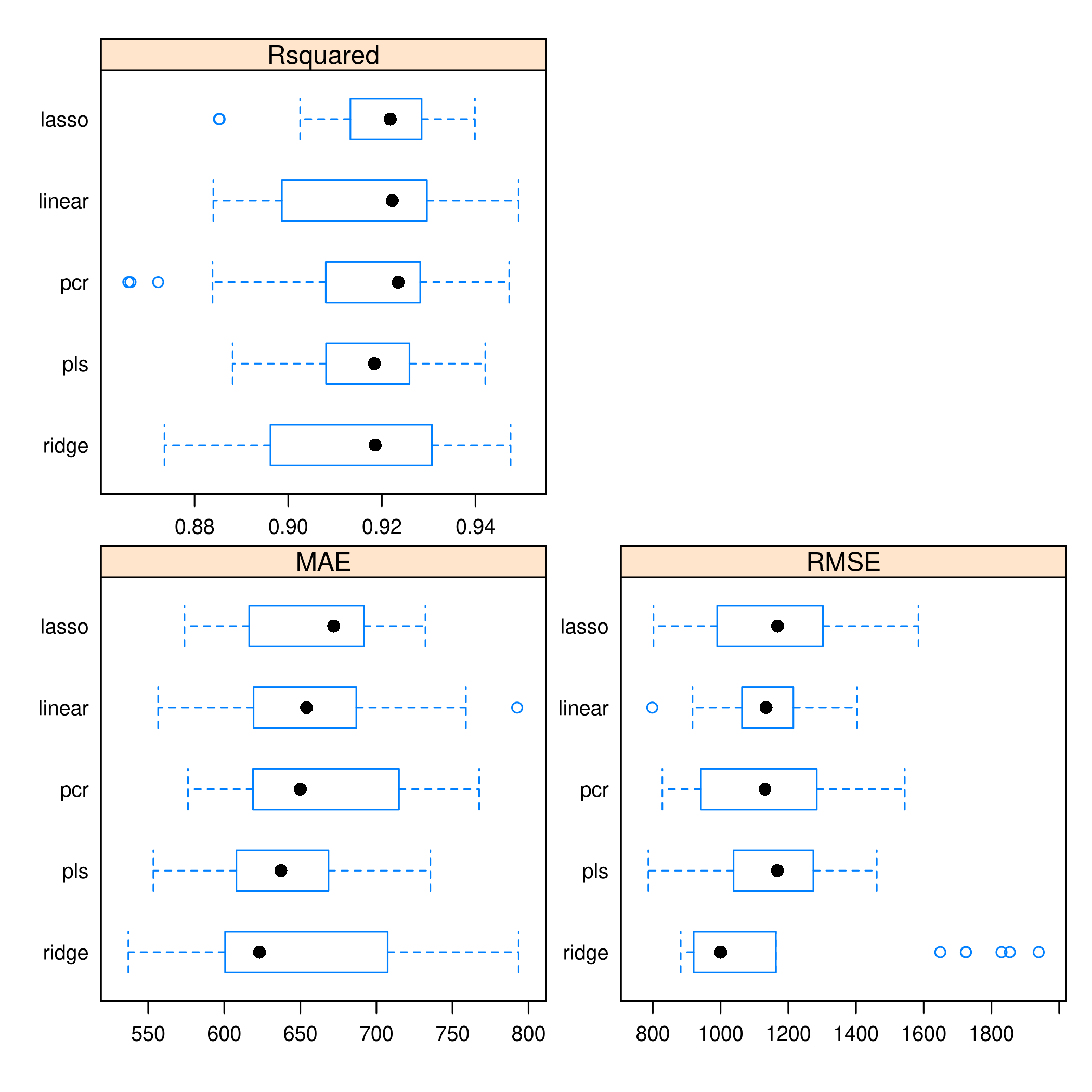
- Given the tighter spread of
PLS, it seems more reliable thanPCR Ridgeis just poor in every wayOLSdoes well, but it also has a worrying outlierLASSOappears to be doing alright as well We also have kept track of the performance on thetest_set
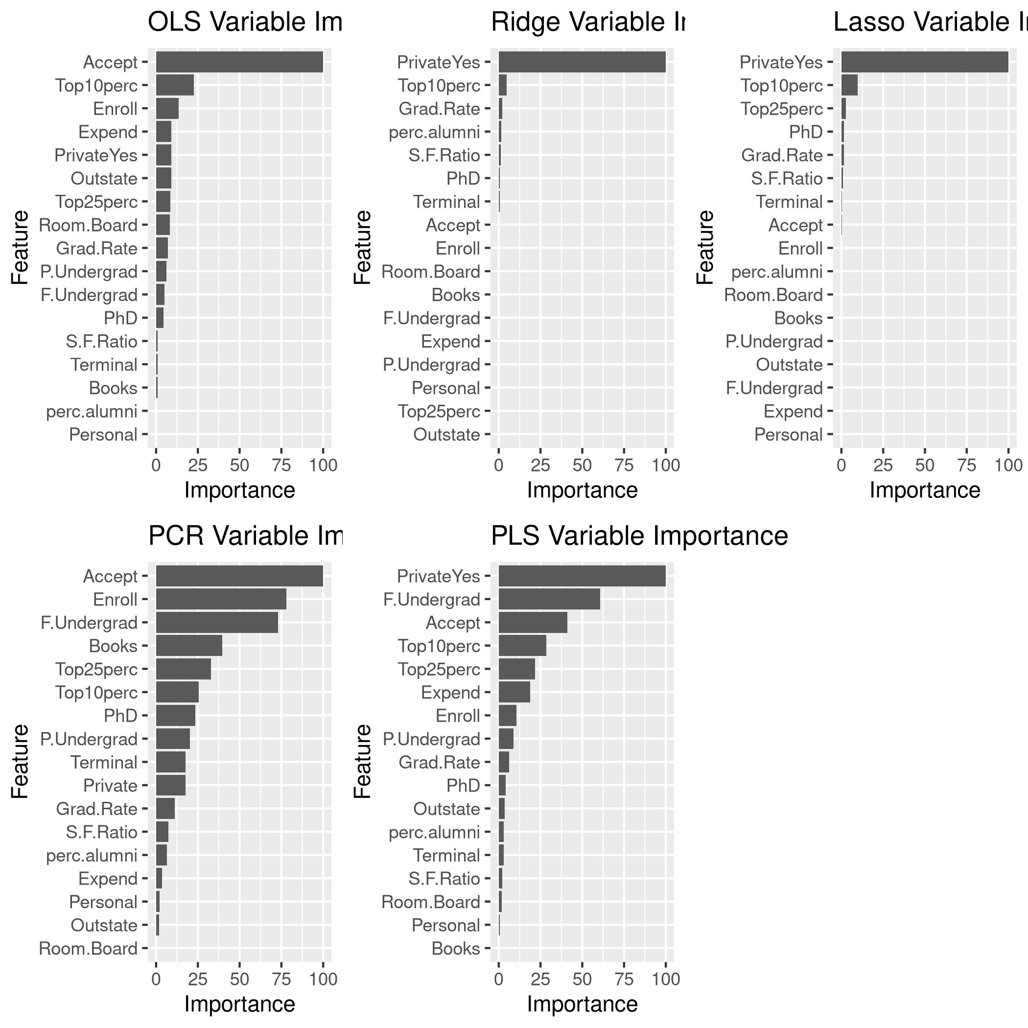
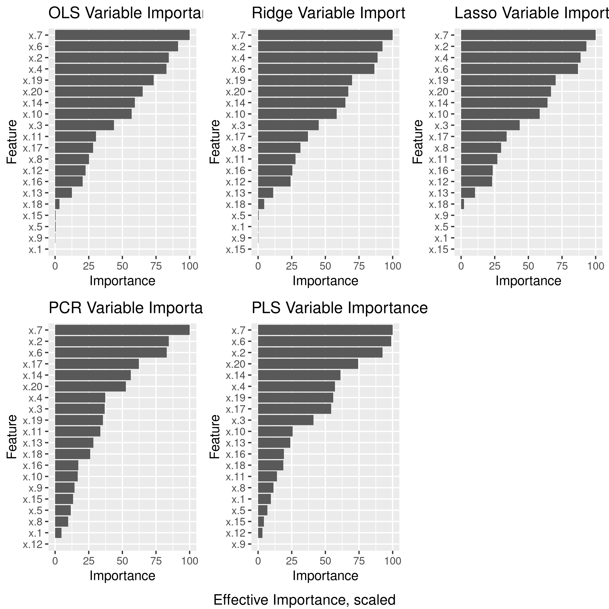
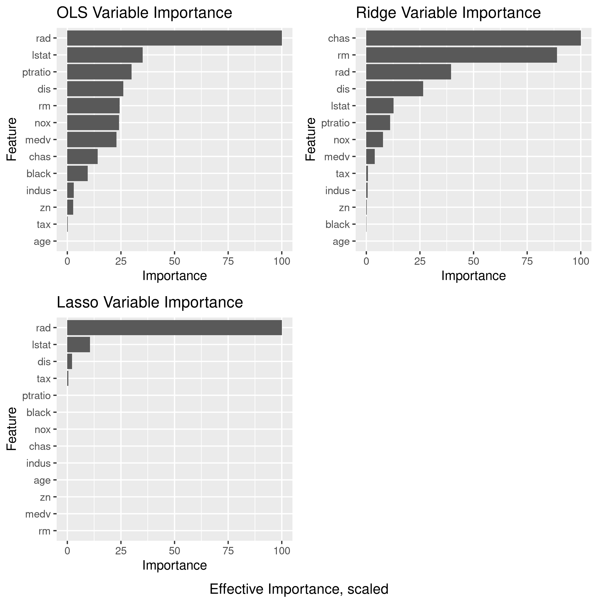
We might want to see the variable significance values as well.
1lgp<-linCol %>% varImp %>% ggplot + ggtitle("OLS Variable Importance")
2rgp<-ridgCol %>% varImp %>% ggplot + ggtitle("Ridge Variable Importance")
3lsgp<-lassoCol %>% varImp %>% ggplot + ggtitle("Lasso Variable Importance")
4pcgp<-pcrCol %>% varImp %>% ggplot + ggtitle("PCR Variable Importance")
5plgp<-plsCol %>% varImp %>% ggplot + ggtitle("PLS Variable Importance")
6grid.arrange(lgp,rgp,lsgp,pcgp,plgp,ncol=3)
Question 6.10 - Pages 263-264
We have seen that as the number of features used in a model increases, the training error will necessarily decrease, but the test error may not. We will now explore this in a simulated data set.
(a) Generate a data set with \(p = 20\) features, \(n = 1,000\) observations, and an associated quantitative response vector generated according to the model \[Y = X\beta + \eta,\] where \(\beta\) has some elements that are exactly equal to zero.
(b) Split your data set into a training set containing \(100\) observations and a test set containing \(900\) observations.
(c) Perform best subset selection on the training set, and plot the training set MSE associated with the best model of each size.
(d) Plot the test set MSE associated with the best model of each size.
(e) For which model size does the test set MSE take on its minimum value? Comment on your results. If it takes on its minimum value for a model containing only an intercept or a model containing all of the features, then play around with the way that you are generating the data in (a) until you come up with a scenario in which the test set MSE is minimized for an intermediate model size.
(f) How does the model at which the test set MSE is minimized compare to the true model used to generate the data? Comment on the coefficient values.
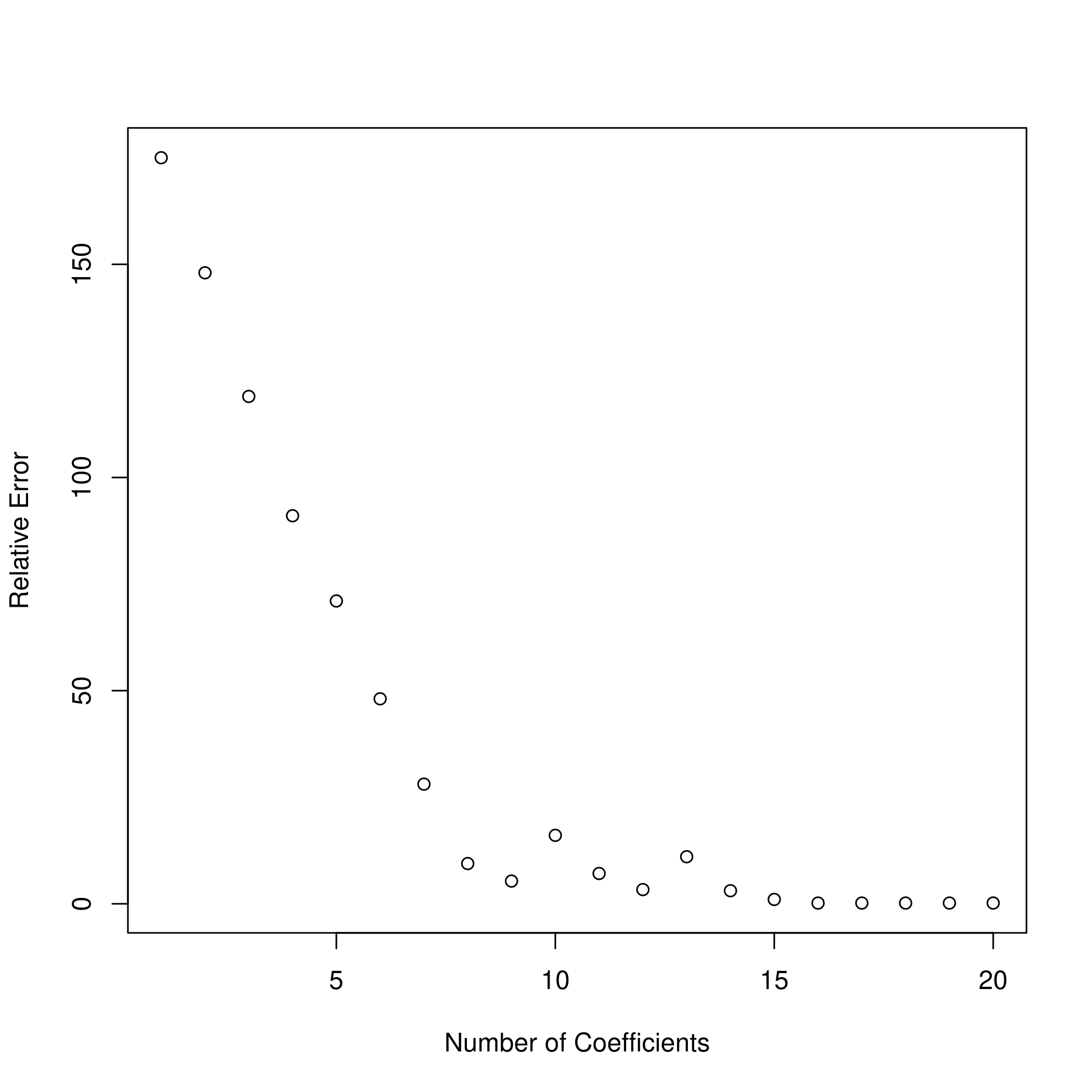
(g) Create a plot displaying \(\sqrt{\Sum_{j=1}^{p}(\beta_{j}-\hat{\beta}_{j}^{r})^{2}}\) for a range of values of \(r\), where \(\hat{\beta}_{j}^{r}\) is the $j$th coefficient estimate for the best model containing \(r\) coefficients. Comment on what you observe. How does this compare to the test MSE plot from (d)?
Answer
Model creation
1p=20
2n=1000
3noise<-rnorm(n)
4xmat<-matrix(rnorm(n*p),nrow=n,ncol=p)
5beta<-sample(-10:34,20)
6beta[sample(1:20,4)]=0
7myY<-xmat %*% beta + noise
8modelDat<-data.frame(x=as.matrix(xmat),y=myY)
- As always we will want to take a peak
1modelDat %>% str %>% print
 1## 'data.frame':    1000 obs. of  21 variables:
 2##  $ x.1 : num  -0.406 -1.375 0.858 -0.231 -0.601 ...
 3##  $ x.2 : num  -0.129 -0.218 -0.17 0.573 -0.513 ...
 4##  $ x.3 : num  0.127 -0.224 1.014 0.896 0.159 ...
 5##  $ x.4 : num  0.499 -0.151 -0.488 -0.959 2.187 ...
 6##  $ x.5 : num  -0.235 -0.345 -0.773 -0.346 0.773 ...
 7##  $ x.6 : num  0.26 -0.429 -1.183 -1.159 0.959 ...
 8##  $ x.7 : num  0.567 1.647 0.149 -0.593 -0.902 ...
 9##  $ x.8 : num  -0.092 0.8391 -1.4835 0.0229 -0.1353 ...
10##  $ x.9 : num  -0.998 -1.043 -0.563 -0.377 0.324 ...
11##  $ x.10: num  -0.4401 -0.195 -0.5139 -0.0156 -0.9543 ...
12##  $ x.11: num  -0.147 0.829 0.165 0.101 -0.105 ...
13##  $ x.12: num  -0.0118 1.02 1.0794 1.3184 -2.2844 ...
14##  $ x.13: num  -1.683 0.487 -1.142 -0.744 -0.175 ...
15##  $ x.14: num  0.228 -1.031 -2.798 -0.646 0.56 ...
16##  $ x.15: num  -0.718 0.508 0.637 -0.556 0.585 ...
17##  $ x.16: num  -1.6378 0.581 -0.9939 0.0537 -0.5854 ...
18##  $ x.17: num  1.758 -0.616 1.377 -0.876 -1.174 ...
19##  $ x.18: num  -1.438 0.373 1.364 0.399 0.949 ...
20##  $ x.19: num  -0.715 -0.731 1.142 0.149 0.916 ...
21##  $ x.20: num  2.774 -2.024 1.316 0.138 0.187 ...
22##  $ y   : num  77.5 -82.8 -38.9 -79.7 64.9 ...
23## NULL
1modelDat %>% summary %>% print
 1##       x.1                x.2                x.3                x.4
 2##  Min.   :-2.79766   Min.   :-3.13281   Min.   :-2.71232   Min.   :-4.29604
 3##  1st Qu.:-0.60516   1st Qu.:-0.66759   1st Qu.:-0.60561   1st Qu.:-0.66598
 4##  Median : 0.04323   Median : 0.03681   Median : 0.06556   Median : 0.06589
 5##  Mean   : 0.06879   Mean   : 0.01004   Mean   : 0.06443   Mean   : 0.02244
 6##  3rd Qu.: 0.74049   3rd Qu.: 0.68234   3rd Qu.: 0.70521   3rd Qu.: 0.71174
 7##  Max.   : 3.50354   Max.   : 3.47268   Max.   : 3.02817   Max.   : 3.27326
 8##       x.5                 x.6                x.7                x.8
 9##  Min.   :-3.228376   Min.   :-4.24014   Min.   :-2.98577   Min.   :-3.27770
10##  1st Qu.:-0.698220   1st Qu.:-0.69448   1st Qu.:-0.59092   1st Qu.:-0.52939
11##  Median :-0.058778   Median :-0.01141   Median : 0.01732   Median : 0.05703
12##  Mean   : 0.000126   Mean   :-0.05158   Mean   : 0.04767   Mean   : 0.08231
13##  3rd Qu.: 0.663570   3rd Qu.: 0.64217   3rd Qu.: 0.67438   3rd Qu.: 0.72849
14##  Max.   : 3.036307   Max.   : 3.27572   Max.   : 2.72163   Max.   : 3.33409
15##       x.9                x.10               x.11               x.12
16##  Min.   :-3.08957   Min.   :-3.21268   Min.   :-3.00572   Min.   :-3.72016
17##  1st Qu.:-0.65456   1st Qu.:-0.69401   1st Qu.:-0.68226   1st Qu.:-0.63043
18##  Median :-0.04242   Median :-0.03069   Median :-0.04777   Median : 0.07079
19##  Mean   : 0.02049   Mean   :-0.02400   Mean   :-0.03729   Mean   : 0.03769
20##  3rd Qu.: 0.71209   3rd Qu.: 0.61540   3rd Qu.: 0.64873   3rd Qu.: 0.67155
21##  Max.   : 3.23110   Max.   : 2.76059   Max.   : 2.87306   Max.   : 3.48569
22##       x.13               x.14               x.15                x.16
23##  Min.   :-3.20126   Min.   :-3.55432   Min.   :-2.857575   Min.   :-3.5383
24##  1st Qu.:-0.68535   1st Qu.:-0.66752   1st Qu.:-0.658708   1st Qu.:-0.7813
25##  Median :-0.01329   Median :-0.03302   Median : 0.020581   Median :-0.0740
26##  Mean   : 0.01094   Mean   : 0.02113   Mean   : 0.007976   Mean   :-0.0883
27##  3rd Qu.: 0.64877   3rd Qu.: 0.74919   3rd Qu.: 0.670464   3rd Qu.: 0.5568
28##  Max.   : 2.78973   Max.   : 3.47923   Max.   : 2.891527   Max.   : 3.0938
29##       x.17               x.18               x.19              x.20
30##  Min.   :-3.28570   Min.   :-4.06416   Min.   :-3.0443   Min.   :-4.06307
31##  1st Qu.:-0.72302   1st Qu.:-0.72507   1st Qu.:-0.6684   1st Qu.:-0.70518
32##  Median :-0.02439   Median :-0.04941   Median :-0.0610   Median :-0.07697
33##  Mean   :-0.01459   Mean   :-0.03164   Mean   :-0.0414   Mean   :-0.05302
34##  3rd Qu.: 0.62692   3rd Qu.: 0.68115   3rd Qu.: 0.6381   3rd Qu.: 0.58597
35##  Max.   : 2.86446   Max.   : 3.32958   Max.   : 3.1722   Max.   : 3.01358
36##        y
37##  Min.   :-199.268
38##  1st Qu.: -54.758
39##  Median :  -1.607
40##  Mean   :  -1.710
41##  3rd Qu.:  49.367
42##  Max.   : 278.244
b) Train Test Split
1train_ind = sample(modelDat %>% nrow,100)
2test_ind = setdiff(seq_len(modelDat %>% nrow), train_set)
Best subset selection
1train_set<-modelDat[train_ind,]
2test_set<-modelDat[-train_ind,]
1linCol<-train(y~.,data=train_set,method="lm")
2linCol %>% summary
 1##
 2## Call:
 3## lm(formula = .outcome ~ ., data = dat)
 4##
 5## Residuals:
 6##      Min       1Q   Median       3Q      Max
 7## -2.12474 -0.53970 -0.00944  0.42398  2.21086
 8##
 9## Coefficients:
10##             Estimate Std. Error  t value Pr(>|t|)
11## (Intercept) -0.06052    0.09604   -0.630    0.530
12## x.1         -0.02265    0.09198   -0.246    0.806
13## x.2         28.91650    0.09879  292.719   <2e-16 ***
14## x.3         14.16532    0.09343  151.610   <2e-16 ***
15## x.4         28.16256    0.09828  286.564   <2e-16 ***
16## x.5          0.13742    0.09658    1.423    0.159
17## x.6         27.01497    0.08540  316.341   <2e-16 ***
18## x.7         31.15917    0.09003  346.092   <2e-16 ***
19## x.8         -9.66308    0.11095  -87.094   <2e-16 ***
20## x.9          0.11641    0.10768    1.081    0.283
21## x.10        19.06687    0.09662  197.344   <2e-16 ***
22## x.11        -9.09956    0.08627 -105.472   <2e-16 ***
23## x.12        -8.01933    0.10198  -78.633   <2e-16 ***
24## x.13         4.26852    0.09888   43.170   <2e-16 ***
25## x.14        20.22366    0.09853  205.247   <2e-16 ***
26## x.15        -0.16607    0.10466   -1.587    0.117
27## x.16         7.95594    0.11250   70.721   <2e-16 ***
28## x.17        10.89851    0.11157   97.684   <2e-16 ***
29## x.18        -1.09760    0.09391  -11.688   <2e-16 ***
30## x.19        22.05197    0.08697  253.553   <2e-16 ***
31## x.20        20.88796    0.09274  225.221   <2e-16 ***
32## ---
33## Signif. codes:  0 '***' 0.001 '**' 0.01 '*' 0.05 '.' 0.1 ' ' 1
34##
35## Residual standard error: 0.8583 on 79 degrees of freedom
36## Multiple R-squared:  0.9999, Adjusted R-squared:  0.9999
37## F-statistic: 4.71e+04 on 20 and 79 DF,  p-value: < 2.2e-16
1linPred<-predict(linCol,test_set)
2linPred %>% postResample(obs = test_set$y)
1##      RMSE  Rsquared       MAE
2## 1.2151815 0.9997265 0.9638378
1L2Grid <- expand.grid(alpha=0,
2                          lambda=10^seq(from=-3,to=30,length=100))
1ridgCol<-train(y~.,data=train_set,method="glmnet",tuneGrid = L2Grid)
1## Warning in nominalTrainWorkflow(x = x, y = y, wts = weights, info = trainInfo, :
2## There were missing values in resampled performance measures.
1ridgCol %>% summary %>% print
 1##             Length Class      Mode
 2## a0           100   -none-     numeric
 3## beta        2000   dgCMatrix  S4
 4## df           100   -none-     numeric
 5## dim            2   -none-     numeric
 6## lambda       100   -none-     numeric
 7## dev.ratio    100   -none-     numeric
 8## nulldev        1   -none-     numeric
 9## npasses        1   -none-     numeric
10## jerr           1   -none-     numeric
11## offset         1   -none-     logical
12## call           5   -none-     call
13## nobs           1   -none-     numeric
14## lambdaOpt      1   -none-     numeric
15## xNames        20   -none-     character
16## problemType    1   -none-     character
17## tuneValue      2   data.frame list
18## obsLevels      1   -none-     logical
19## param          0   -none-     list
1coef(ridgCol$finalModel, ridgCol$bestTune$lambda) %>% print
 1## 21 x 1 sparse Matrix of class "dgCMatrix"
 2##                       1
 3## (Intercept)  0.03898376
 4## x.1         -0.12140945
 5## x.2         27.63771674
 6## x.3         13.46853844
 7## x.4         26.54402352
 8## x.5         -0.13838118
 9## x.6         25.87706885
10## x.7         29.90687677
11## x.8         -9.42088971
12## x.9         -0.08983349
13## x.10        17.45444598
14## x.11        -8.33991071
15## x.12        -7.23653865
16## x.13         3.35145521
17## x.14        19.42178898
18## x.15        -0.02794731
19## x.16         7.63951382
20## x.17        11.08083907
21## x.18        -1.36872894
22## x.19        20.90257005
23## x.20        20.07494414
1ggplot(ridgCol)
1ridgPred<-predict(ridgCol,test_set)
2ridgPred %>% postResample(obs = test_set$y)
1##      RMSE  Rsquared       MAE
2## 3.7554417 0.9994231 3.0184859
1L1Grid <- expand.grid(alpha=1, # for lasso
2                          lambda=10^seq(from=-3,to=30,length=100))
1lassoCol<-train(y~.,data=train_set,method="glmnet",tuneGrid = L1Grid)
1## Warning in nominalTrainWorkflow(x = x, y = y, wts = weights, info = trainInfo, :
2## There were missing values in resampled performance measures.
1lassoCol %>% summary %>% print
 1##             Length Class      Mode
 2## a0           47    -none-     numeric
 3## beta        940    dgCMatrix  S4
 4## df           47    -none-     numeric
 5## dim           2    -none-     numeric
 6## lambda       47    -none-     numeric
 7## dev.ratio    47    -none-     numeric
 8## nulldev       1    -none-     numeric
 9## npasses       1    -none-     numeric
10## jerr          1    -none-     numeric
11## offset        1    -none-     logical
12## call          5    -none-     call
13## nobs          1    -none-     numeric
14## lambdaOpt     1    -none-     numeric
15## xNames       20    -none-     character
16## problemType   1    -none-     character
17## tuneValue     2    data.frame list
18## obsLevels     1    -none-     logical
19## param         0    -none-     list
1coef(lassoCol$finalModel, lassoCol$bestTune$lambda) %>% print
 1## 21 x 1 sparse Matrix of class "dgCMatrix"
 2##                      1
 3## (Intercept)  0.1158884
 4## x.1          .
 5## x.2         28.5897869
 6## x.3         13.3637110
 7## x.4         27.2558797
 8## x.5          .
 9## x.6         26.6625588
10## x.7         30.6841774
11## x.8         -9.1388677
12## x.9          .
13## x.10        17.9220939
14## x.11        -8.2461257
15## x.12        -7.0603651
16## x.13         3.2052101
17## x.14        19.7219890
18## x.15         .
19## x.16         7.2082509
20## x.17        10.4137411
21## x.18        -0.6693664
22## x.19        21.5357460
23## x.20        20.5226071
1ggplot(lassoCol)
1lassoPred<-predict(lassoCol,test_set)
2lassoPred %>% postResample(obs = test_set$y)
1##      RMSE  Rsquared       MAE
2## 2.7289452 0.9992454 2.2029482
1mGrid <- expand.grid(ncomp=seq(from=1,to=20,length=10))
1pcrCol<-train(y~.,data=train_set,method="pcr",tuneGrid = mGrid)
2pcrCol %>% summary %>% print
 1## Data:    X dimension: 100 20
 2##  Y dimension: 100 1
 3## Fit method: svdpc
 4## Number of components considered: 20
 5## TRAINING: % variance explained
 6##           1 comps  2 comps  3 comps  4 comps  5 comps  6 comps  7 comps
 7## X          10.040    18.46    26.62    34.56    41.87    48.54    54.56
 8## .outcome    8.425    34.90    41.09    43.12    45.06    48.09    66.44
 9##           8 comps  9 comps  10 comps  11 comps  12 comps  13 comps  14 comps
10## X           60.33    65.37     70.01     74.46     78.72     82.32     85.67
11## .outcome    85.76    88.81     89.93     91.66     91.91     92.04     92.08
12##           15 comps  16 comps  17 comps  18 comps  19 comps  20 comps
13## X            88.85     91.94     94.59     96.73     98.51    100.00
14## .outcome     92.15     94.96     99.51     99.57     99.76     99.99
15## NULL
1ggplot(pcrCol)
1pcrPred<-predict(pcrCol,test_set)
2pcrPred %>% postResample(obs = test_set$y)
1##      RMSE  Rsquared       MAE
2## 1.2151815 0.9997265 0.9638378
1plsCol<-train(y~.,data=train_set,method="pls",tuneGrid = mGrid)
2plsCol %>% summary %>% print
 1## Data:    X dimension: 100 20
 2##  Y dimension: 100 1
 3## Fit method: oscorespls
 4## Number of components considered: 20
 5## TRAINING: % variance explained
 6##           1 comps  2 comps  3 comps  4 comps  5 comps  6 comps  7 comps
 7## X           7.762    14.79    21.01    26.89    31.55    36.13    41.12
 8## .outcome   92.765    98.81    99.75    99.96    99.98    99.99    99.99
 9##           8 comps  9 comps  10 comps  11 comps  12 comps  13 comps  14 comps
10## X           46.35    51.21     56.12     60.34     65.63     71.57     76.16
11## .outcome    99.99    99.99     99.99     99.99     99.99     99.99     99.99
12##           15 comps  16 comps  17 comps  18 comps  19 comps  20 comps
13## X            80.72     84.69     88.98     92.69     96.71    100.00
14## .outcome     99.99     99.99     99.99     99.99     99.99     99.99
15## NULL
1ggplot(plsCol)
1plsPred<-predict(plsCol,test_set)
2plsPred %>% postResample(obs = test_set$y)
1##      RMSE  Rsquared       MAE
2## 1.2151815 0.9997265 0.9638378
d) Test MSE for best models
- All the models have the same R² but Ridge does the worst followed by LASSO
For the rest of the question, we will consider the OLS model.
1modelFit<-regsubsets(y~.,data=modelDat,nvmax=20)
2modelFit %>% summary %>% print
 1## Subset selection object
 2## Call: regsubsets.formula(y ~ ., data = modelDat, nvmax = 20)
 3## 20 Variables  (and intercept)
 4##      Forced in Forced out
 5## x.1      FALSE      FALSE
 6## x.2      FALSE      FALSE
 7## x.3      FALSE      FALSE
 8## x.4      FALSE      FALSE
 9## x.5      FALSE      FALSE
10## x.6      FALSE      FALSE
11## x.7      FALSE      FALSE
12## x.8      FALSE      FALSE
13## x.9      FALSE      FALSE
14## x.10     FALSE      FALSE
15## x.11     FALSE      FALSE
16## x.12     FALSE      FALSE
17## x.13     FALSE      FALSE
18## x.14     FALSE      FALSE
19## x.15     FALSE      FALSE
20## x.16     FALSE      FALSE
21## x.17     FALSE      FALSE
22## x.18     FALSE      FALSE
23## x.19     FALSE      FALSE
24## x.20     FALSE      FALSE
25## 1 subsets of each size up to 20
26## Selection Algorithm: exhaustive
27##           x.1 x.2 x.3 x.4 x.5 x.6 x.7 x.8 x.9 x.10 x.11 x.12 x.13 x.14 x.15
28## 1  ( 1 )  " " " " " " " " " " " " "*" " " " " " "  " "  " "  " "  " "  " "
29## 2  ( 1 )  " " " " " " " " " " "*" "*" " " " " " "  " "  " "  " "  " "  " "
30## 3  ( 1 )  " " "*" " " " " " " "*" "*" " " " " " "  " "  " "  " "  " "  " "
31## 4  ( 1 )  " " "*" " " "*" " " "*" "*" " " " " " "  " "  " "  " "  " "  " "
32## 5  ( 1 )  " " "*" " " "*" " " "*" "*" " " " " " "  " "  " "  " "  "*"  " "
33## 6  ( 1 )  " " "*" " " "*" " " "*" "*" " " " " " "  " "  " "  " "  " "  " "
34## 7  ( 1 )  " " "*" " " "*" " " "*" "*" " " " " " "  " "  " "  " "  "*"  " "
35## 8  ( 1 )  " " "*" " " "*" " " "*" "*" " " " " "*"  " "  " "  " "  "*"  " "
36## 9  ( 1 )  " " "*" "*" "*" " " "*" "*" " " " " "*"  " "  " "  " "  "*"  " "
37## 10  ( 1 ) " " "*" "*" "*" " " "*" "*" " " " " "*"  " "  " "  " "  "*"  " "
38## 11  ( 1 ) " " "*" "*" "*" " " "*" "*" " " " " "*"  "*"  " "  " "  "*"  " "
39## 12  ( 1 ) " " "*" "*" "*" " " "*" "*" "*" " " "*"  "*"  " "  " "  "*"  " "
40## 13  ( 1 ) " " "*" "*" "*" " " "*" "*" "*" " " "*"  "*"  "*"  " "  "*"  " "
41## 14  ( 1 ) " " "*" "*" "*" " " "*" "*" "*" " " "*"  "*"  "*"  " "  "*"  " "
42## 15  ( 1 ) " " "*" "*" "*" " " "*" "*" "*" " " "*"  "*"  "*"  "*"  "*"  " "
43## 16  ( 1 ) " " "*" "*" "*" " " "*" "*" "*" " " "*"  "*"  "*"  "*"  "*"  " "
44## 17  ( 1 ) "*" "*" "*" "*" " " "*" "*" "*" " " "*"  "*"  "*"  "*"  "*"  " "
45## 18  ( 1 ) "*" "*" "*" "*" " " "*" "*" "*" " " "*"  "*"  "*"  "*"  "*"  "*"
46## 19  ( 1 ) "*" "*" "*" "*" "*" "*" "*" "*" " " "*"  "*"  "*"  "*"  "*"  "*"
47## 20  ( 1 ) "*" "*" "*" "*" "*" "*" "*" "*" "*" "*"  "*"  "*"  "*"  "*"  "*"
48##           x.16 x.17 x.18 x.19 x.20
49## 1  ( 1 )  " "  " "  " "  " "  " "
50## 2  ( 1 )  " "  " "  " "  " "  " "
51## 3  ( 1 )  " "  " "  " "  " "  " "
52## 4  ( 1 )  " "  " "  " "  " "  " "
53## 5  ( 1 )  " "  " "  " "  " "  " "
54## 6  ( 1 )  " "  " "  " "  "*"  "*"
55## 7  ( 1 )  " "  " "  " "  "*"  "*"
56## 8  ( 1 )  " "  " "  " "  "*"  "*"
57## 9  ( 1 )  " "  " "  " "  "*"  "*"
58## 10  ( 1 ) " "  "*"  " "  "*"  "*"
59## 11  ( 1 ) " "  "*"  " "  "*"  "*"
60## 12  ( 1 ) " "  "*"  " "  "*"  "*"
61## 13  ( 1 ) " "  "*"  " "  "*"  "*"
62## 14  ( 1 ) "*"  "*"  " "  "*"  "*"
63## 15  ( 1 ) "*"  "*"  " "  "*"  "*"
64## 16  ( 1 ) "*"  "*"  "*"  "*"  "*"
65## 17  ( 1 ) "*"  "*"  "*"  "*"  "*"
66## 18  ( 1 ) "*"  "*"  "*"  "*"  "*"
67## 19  ( 1 ) "*"  "*"  "*"  "*"  "*"
68## 20  ( 1 ) "*"  "*"  "*"  "*"  "*"
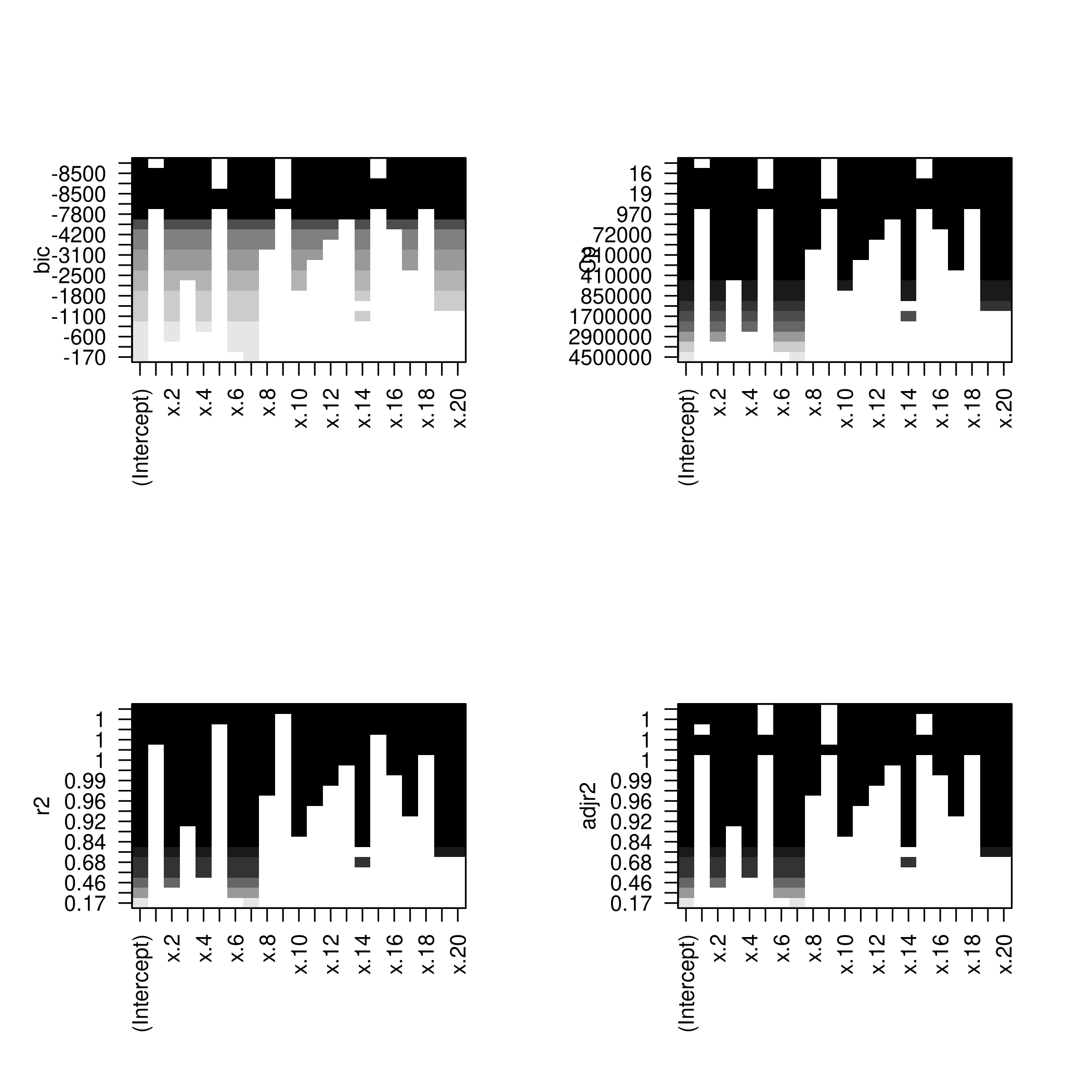
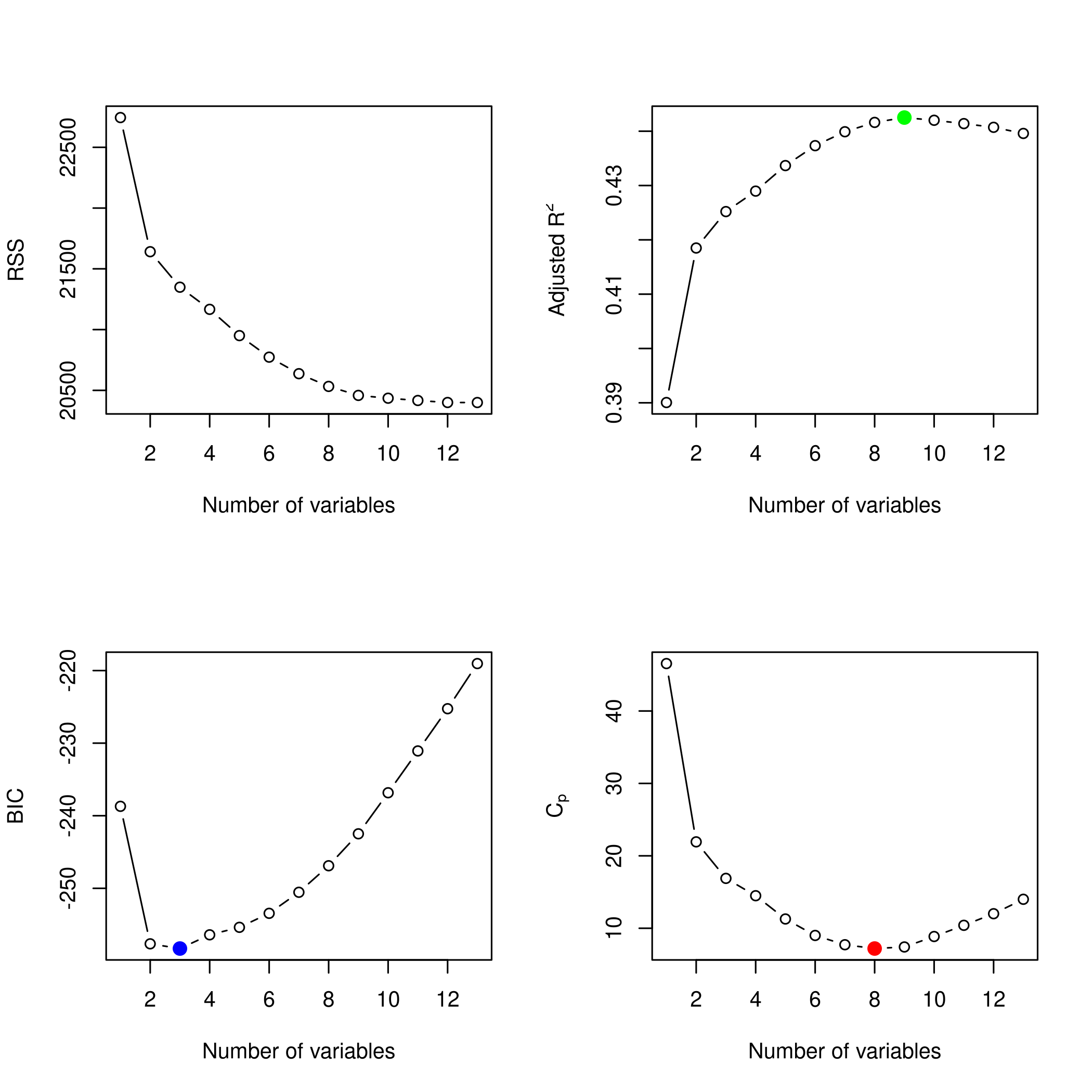
We might want to take a look at these.
1par(mfrow=c(2,2))
2plot(modelFit)
3plot(modelFit,scale='Cp')
4plot(modelFit,scale='r2')
5plot(modelFit,scale='adjr2')
1plotLEAP(modelFit %>% summary)
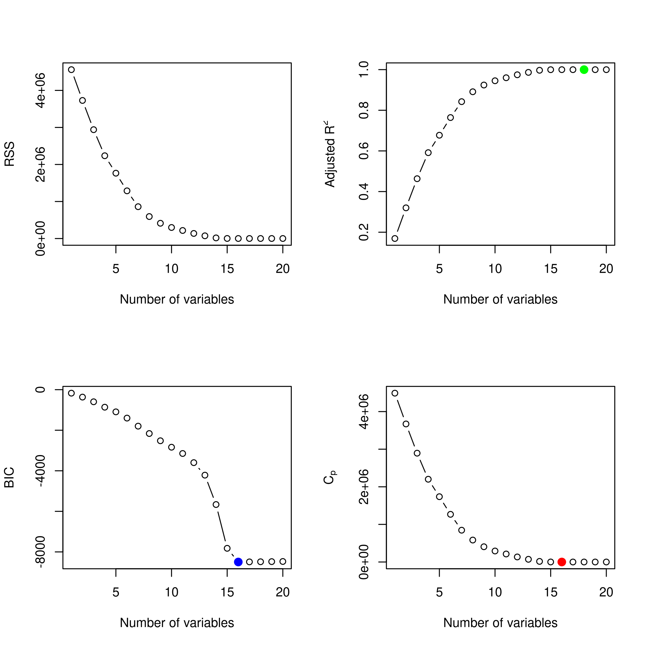
It would appear that 16 variables would be a good bet. We note that the lasso model did void out 4 parameters, namely x₁,x₃,x₁₃ and x₁₇.
Lets take a quick look at the various model variable significance values.
1lgp<-linCol %>% varImp %>% ggplot + ggtitle("OLS Variable Importance")
2rgp<-ridgCol %>% varImp %>% ggplot + ggtitle("Ridge Variable Importance")
3lsgp<-lassoCol %>% varImp %>% ggplot + ggtitle("Lasso Variable Importance")
4pcgp<-pcrCol %>% varImp %>% ggplot + ggtitle("PCR Variable Importance")
5plgp<-plsCol %>% varImp %>% ggplot + ggtitle("PLS Variable Importance")
6grid.arrange(lgp,rgp,lsgp,pcgp,plgp,ncol=3,bottom="Effective Importance, scaled")
e) Model size
The test set numeric minimum RMSE is a tie between OLS and PCR, and this was achieved for the (effective) 16 variable OLS model, as well as the 18 variable PCR model.
f) Best model
We will consider the OLS and PCR models and its parameters.
1linCol$finalModel %>% print
 1##
 2## Call:
 3## lm(formula = .outcome ~ ., data = dat)
 4##
 5## Coefficients:
 6## (Intercept)          x.1          x.2          x.3          x.4          x.5
 7##    -0.06052     -0.02265     28.91650     14.16532     28.16256      0.13742
 8##         x.6          x.7          x.8          x.9         x.10         x.11
 9##    27.01497     31.15917     -9.66308      0.11641     19.06687     -9.09956
10##        x.12         x.13         x.14         x.15         x.16         x.17
11##    -8.01933      4.26852     20.22366     -0.16607      7.95594     10.89851
12##        x.18         x.19         x.20
13##    -1.09760     22.05197     20.88796
1pcrCol$bestTune %>% print
1##    ncomp
2## 10    20
Now to compare this to the original.
1beta %>% print
1##  [1]   0  29  14  28   0  27  31 -10   0  19  -9  -8   4  20   0   8  11  -1  22
2## [20]  21
1t=data.frame(linCol$finalModel$coefficients[-1]) %>% rename("Model_Coeffs"=1) %>% add_column(beta) %>% rename("Original_Coeffs"=2)
2print(t)
 1##      Model_Coeffs Original_Coeffs
 2## x.1   -0.02265289               0
 3## x.2   28.91649699              29
 4## x.3   14.16532050              14
 5## x.4   28.16255937              28
 6## x.5    0.13741621               0
 7## x.6   27.01497459              27
 8## x.7   31.15917172              31
 9## x.8   -9.66308362             -10
10## x.9    0.11641282               0
11## x.10  19.06687041              19
12## x.11  -9.09955826              -9
13## x.12  -8.01932598              -8
14## x.13   4.26852334               4
15## x.14  20.22366153              20
16## x.15  -0.16606531               0
17## x.16   7.95593559               8
18## x.17  10.89851353              11
19## x.18  -1.09759687              -1
20## x.19  22.05196537              22
21## x.20  20.88795623              21
We see that the coefficients are pretty similar.
g) Plotting differences
 1val.errors = rep(NaN, p)
 2a = rep(NaN, p)
 3b = rep(NaN, p)
 4x_cols = colnames(xmat, do.NULL = FALSE, prefix = "x.")
 5for (i in 1:p) {
 6    coefi = coef(modelFit, id = i)
 7    a[i] = length(coefi) - 1 ## Not counting the intercept
 8    b[i] = sqrt(sum((beta[x_cols %in% names(coefi)] - coefi[names(coefi) %in% x_cols])^2) +
 9        sum(beta[!(x_cols %in% names(coefi))])^2) ## Handling the intercept
10}
11plot(x = a, y = b, xlab = "Number of Coefficients", ylab = "Relative Error")
Question 6.11 - Page 264
We will now try to predict per capita crime rate in the Boston data set.
(a) Try out some of the regression methods explored in this chapter, such as best subset selection, the lasso, ridge regression, and PCR. Present and discuss results for the approaches that you consider.
(b) Propose a model (or set of models) that seem to perform well on this data set, and justify your answer. Make sure that you are evaluating model performance using validation set error, crossvalidation, or some other reasonable alternative, as opposed to using training error.
(c) Does your chosen model involve all of the features in the data set? Why or why not?
Answer
1boston<-MASS::Boston
- Summarize
1boston %>% str %>% print
 1## 'data.frame':    506 obs. of  14 variables:
 2##  $ crim   : num  0.00632 0.02731 0.02729 0.03237 0.06905 ...
 3##  $ zn     : num  18 0 0 0 0 0 12.5 12.5 12.5 12.5 ...
 4##  $ indus  : num  2.31 7.07 7.07 2.18 2.18 2.18 7.87 7.87 7.87 7.87 ...
 5##  $ chas   : int  0 0 0 0 0 0 0 0 0 0 ...
 6##  $ nox    : num  0.538 0.469 0.469 0.458 0.458 0.458 0.524 0.524 0.524 0.524 ...
 7##  $ rm     : num  6.58 6.42 7.18 7 7.15 ...
 8##  $ age    : num  65.2 78.9 61.1 45.8 54.2 58.7 66.6 96.1 100 85.9 ...
 9##  $ dis    : num  4.09 4.97 4.97 6.06 6.06 ...
10##  $ rad    : int  1 2 2 3 3 3 5 5 5 5 ...
11##  $ tax    : num  296 242 242 222 222 222 311 311 311 311 ...
12##  $ ptratio: num  15.3 17.8 17.8 18.7 18.7 18.7 15.2 15.2 15.2 15.2 ...
13##  $ black  : num  397 397 393 395 397 ...
14##  $ lstat  : num  4.98 9.14 4.03 2.94 5.33 ...
15##  $ medv   : num  24 21.6 34.7 33.4 36.2 28.7 22.9 27.1 16.5 18.9 ...
16## NULL
1boston %>% summary %>% print
 1##       crim                zn             indus            chas
 2##  Min.   : 0.00632   Min.   :  0.00   Min.   : 0.46   Min.   :0.00000
 3##  1st Qu.: 0.08204   1st Qu.:  0.00   1st Qu.: 5.19   1st Qu.:0.00000
 4##  Median : 0.25651   Median :  0.00   Median : 9.69   Median :0.00000
 5##  Mean   : 3.61352   Mean   : 11.36   Mean   :11.14   Mean   :0.06917
 6##  3rd Qu.: 3.67708   3rd Qu.: 12.50   3rd Qu.:18.10   3rd Qu.:0.00000
 7##  Max.   :88.97620   Max.   :100.00   Max.   :27.74   Max.   :1.00000
 8##       nox               rm             age              dis
 9##  Min.   :0.3850   Min.   :3.561   Min.   :  2.90   Min.   : 1.130
10##  1st Qu.:0.4490   1st Qu.:5.886   1st Qu.: 45.02   1st Qu.: 2.100
11##  Median :0.5380   Median :6.208   Median : 77.50   Median : 3.207
12##  Mean   :0.5547   Mean   :6.285   Mean   : 68.57   Mean   : 3.795
13##  3rd Qu.:0.6240   3rd Qu.:6.623   3rd Qu.: 94.08   3rd Qu.: 5.188
14##  Max.   :0.8710   Max.   :8.780   Max.   :100.00   Max.   :12.127
15##       rad              tax           ptratio          black
16##  Min.   : 1.000   Min.   :187.0   Min.   :12.60   Min.   :  0.32
17##  1st Qu.: 4.000   1st Qu.:279.0   1st Qu.:17.40   1st Qu.:375.38
18##  Median : 5.000   Median :330.0   Median :19.05   Median :391.44
19##  Mean   : 9.549   Mean   :408.2   Mean   :18.46   Mean   :356.67
20##  3rd Qu.:24.000   3rd Qu.:666.0   3rd Qu.:20.20   3rd Qu.:396.23
21##  Max.   :24.000   Max.   :711.0   Max.   :22.00   Max.   :396.90
22##      lstat            medv
23##  Min.   : 1.73   Min.   : 5.00
24##  1st Qu.: 6.95   1st Qu.:17.02
25##  Median :11.36   Median :21.20
26##  Mean   :12.65   Mean   :22.53
27##  3rd Qu.:16.95   3rd Qu.:25.00
28##  Max.   :37.97   Max.   :50.00
1boston %>% sapply(unique) %>% sapply(length) %>% print
1##    crim      zn   indus    chas     nox      rm     age     dis     rad     tax
2##     504      26      76       2      81     446     356     412       9      66
3## ptratio   black   lstat    medv
4##      46     357     455     229
a) Test regression models
1train_ind = sample(boston %>% nrow,100)
2test_ind = setdiff(seq_len(boston %>% nrow), train_set)
1train_set<-boston[train_ind,]
2test_set<-boston[-train_ind,]
1linCol<-train(crim~.,data=train_set,method="lm")
2linCol %>% summary
 1##
 2## Call:
 3## lm(formula = .outcome ~ ., data = dat)
 4##
 5## Residuals:
 6##     Min      1Q  Median      3Q     Max
 7## -6.2431 -1.0344 -0.0563  0.8187  8.1318
 8##
 9## Coefficients:
10##               Estimate Std. Error t value Pr(>|t|)
11## (Intercept)  0.9339246  7.6508393   0.122   0.9031
12## zn           0.0046819  0.0157375   0.297   0.7668
13## indus        0.0276209  0.0875254   0.316   0.7531
14## chas        -1.1602278  1.2386869  -0.937   0.3516
15## nox         -7.5024503  5.0207818  -1.494   0.1388
16## rm           1.1240874  0.7462340   1.506   0.1356
17## age          0.0020182  0.0137404   0.147   0.8836
18## dis         -0.3934753  0.2454365  -1.603   0.1126
19## rad          0.4540613  0.0791580   5.736 1.41e-07 ***
20## tax          0.0008469  0.0052593   0.161   0.8724
21## ptratio     -0.2978204  0.1637629  -1.819   0.0725 .
22## black        0.0030642  0.0045281   0.677   0.5004
23## lstat        0.1322779  0.0626485   2.111   0.0376 *
24## medv        -0.0841382  0.0590700  -1.424   0.1580
25## ---
26## Signif. codes:  0 '***' 0.001 '**' 0.01 '*' 0.05 '.' 0.1 ' ' 1
27##
28## Residual standard error: 2.362 on 86 degrees of freedom
29## Multiple R-squared:  0.775,  Adjusted R-squared:  0.741
30## F-statistic: 22.78 on 13 and 86 DF,  p-value: < 2.2e-16
1linPred<-predict(linCol,test_set)
2linPred %>% postResample(obs = test_set$crim)
1##      RMSE  Rsquared       MAE
2## 7.3794735 0.4056002 2.6774969
1L2Grid <- expand.grid(alpha=0,
2                          lambda=10^seq(from=-3,to=30,length=100))
1ridgCol<-train(crim~.,data=train_set,method="glmnet",tuneGrid = L2Grid)
1## Warning in nominalTrainWorkflow(x = x, y = y, wts = weights, info = trainInfo, :
2## There were missing values in resampled performance measures.
1ridgCol %>% summary %>% print
 1##             Length Class      Mode
 2## a0           100   -none-     numeric
 3## beta        1300   dgCMatrix  S4
 4## df           100   -none-     numeric
 5## dim            2   -none-     numeric
 6## lambda       100   -none-     numeric
 7## dev.ratio    100   -none-     numeric
 8## nulldev        1   -none-     numeric
 9## npasses        1   -none-     numeric
10## jerr           1   -none-     numeric
11## offset         1   -none-     logical
12## call           5   -none-     call
13## nobs           1   -none-     numeric
14## lambdaOpt      1   -none-     numeric
15## xNames        13   -none-     character
16## problemType    1   -none-     character
17## tuneValue      2   data.frame list
18## obsLevels      1   -none-     logical
19## param          0   -none-     list
1coef(ridgCol$finalModel, ridgCol$bestTune$lambda) %>% print
 1## 14 x 1 sparse Matrix of class "dgCMatrix"
 2##                        1
 3## (Intercept) -3.881166065
 4## zn           0.002597790
 5## indus       -0.005103517
 6## chas        -0.674764337
 7## nox         -0.053645732
 8## rm           0.600064844
 9## age          0.001153570
10## dis         -0.179295384
11## rad          0.267082956
12## tax          0.006447932
13## ptratio     -0.075885753
14## black       -0.001650403
15## lstat        0.086462700
16## medv        -0.027519270
1ggplot(ridgCol)

1ridgPred<-predict(ridgCol,test_set)
2ridgPred %>% postResample(obs = test_set$crim)
1##      RMSE  Rsquared       MAE
2## 7.5065916 0.4017056 2.4777547
1L1Grid <- expand.grid(alpha=1, # for lasso
2                          lambda=10^seq(from=-3,to=30,length=100))
1lassoCol<-train(crim~.,data=train_set,method="glmnet",tuneGrid = L1Grid)
1## Warning in nominalTrainWorkflow(x = x, y = y, wts = weights, info = trainInfo, :
2## There were missing values in resampled performance measures.
1lassoCol %>% summary %>% print
 1##             Length Class      Mode
 2## a0            78   -none-     numeric
 3## beta        1014   dgCMatrix  S4
 4## df            78   -none-     numeric
 5## dim            2   -none-     numeric
 6## lambda        78   -none-     numeric
 7## dev.ratio     78   -none-     numeric
 8## nulldev        1   -none-     numeric
 9## npasses        1   -none-     numeric
10## jerr           1   -none-     numeric
11## offset         1   -none-     logical
12## call           5   -none-     call
13## nobs           1   -none-     numeric
14## lambdaOpt      1   -none-     numeric
15## xNames        13   -none-     character
16## problemType    1   -none-     character
17## tuneValue      2   data.frame list
18## obsLevels      1   -none-     logical
19## param          0   -none-     list
1coef(lassoCol$finalModel, lassoCol$bestTune$lambda) %>% print
 1## 14 x 1 sparse Matrix of class "dgCMatrix"
 2##                        1
 3## (Intercept) -2.024006430
 4## zn           .
 5## indus        .
 6## chas         .
 7## nox          .
 8## rm           .
 9## age          .
10## dis         -0.008506188
11## rad          0.386379255
12## tax          0.001779579
13## ptratio      .
14## black        .
15## lstat        0.040788606
16## medv         .
1ggplot(lassoCol)

1lassoPred<-predict(lassoCol,test_set)
2lassoPred %>% postResample(obs = test_set$crim)
1##      RMSE  Rsquared       MAE
2## 7.5868293 0.3859121 2.4892258
1mGrid <- expand.grid(ncomp=seq(from=1,to=20,length=10))
- All the models have the same R² but Ridge does the worst followed by LASSO
For the rest of the question, we will consider the OLS model.
1modelFit<-regsubsets(crim~.,data=boston,nvmax=20)
2modelFit %>% summary %>% print
 1## Subset selection object
 2## Call: regsubsets.formula(crim ~ ., data = boston, nvmax = 20)
 3## 13 Variables  (and intercept)
 4##         Forced in Forced out
 5## zn          FALSE      FALSE
 6## indus       FALSE      FALSE
 7## chas        FALSE      FALSE
 8## nox         FALSE      FALSE
 9## rm          FALSE      FALSE
10## age         FALSE      FALSE
11## dis         FALSE      FALSE
12## rad         FALSE      FALSE
13## tax         FALSE      FALSE
14## ptratio     FALSE      FALSE
15## black       FALSE      FALSE
16## lstat       FALSE      FALSE
17## medv        FALSE      FALSE
18## 1 subsets of each size up to 13
19## Selection Algorithm: exhaustive
20##           zn  indus chas nox rm  age dis rad tax ptratio black lstat medv
21## 1  ( 1 )  " " " "   " "  " " " " " " " " "*" " " " "     " "   " "   " "
22## 2  ( 1 )  " " " "   " "  " " " " " " " " "*" " " " "     " "   "*"   " "
23## 3  ( 1 )  " " " "   " "  " " " " " " " " "*" " " " "     "*"   "*"   " "
24## 4  ( 1 )  "*" " "   " "  " " " " " " "*" "*" " " " "     " "   " "   "*"
25## 5  ( 1 )  "*" " "   " "  " " " " " " "*" "*" " " " "     "*"   " "   "*"
26## 6  ( 1 )  "*" " "   " "  "*" " " " " "*" "*" " " " "     "*"   " "   "*"
27## 7  ( 1 )  "*" " "   " "  "*" " " " " "*" "*" " " "*"     "*"   " "   "*"
28## 8  ( 1 )  "*" " "   " "  "*" " " " " "*" "*" " " "*"     "*"   "*"   "*"
29## 9  ( 1 )  "*" "*"   " "  "*" " " " " "*" "*" " " "*"     "*"   "*"   "*"
30## 10  ( 1 ) "*" "*"   " "  "*" "*" " " "*" "*" " " "*"     "*"   "*"   "*"
31## 11  ( 1 ) "*" "*"   " "  "*" "*" " " "*" "*" "*" "*"     "*"   "*"   "*"
32## 12  ( 1 ) "*" "*"   "*"  "*" "*" " " "*" "*" "*" "*"     "*"   "*"   "*"
33## 13  ( 1 ) "*" "*"   "*"  "*" "*" "*" "*" "*" "*" "*"     "*"   "*"   "*"
We might want to take a look at these.
1par(mfrow=c(2,2))
2plot(modelFit)
3plot(modelFit,scale='Cp')
4plot(modelFit,scale='r2')
5plot(modelFit,scale='adjr2')
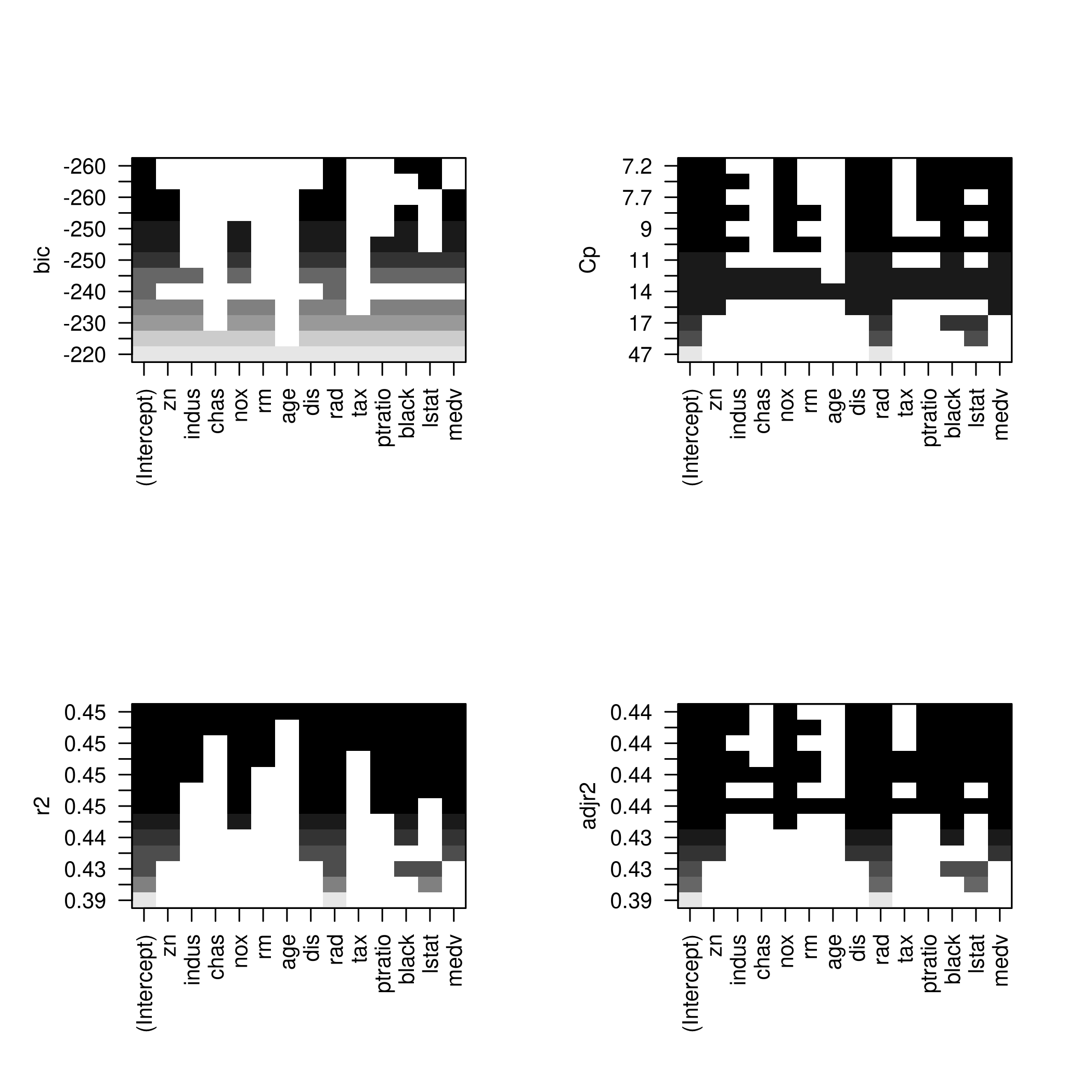
1plotLEAP(modelFit %>% summary)
It would appear that 16 variables would be a good bet. We note that the lasso model did void out 4 parameters, namely x₁,x₃,x₁₃ and x₁₇.
Lets take a quick look at the various model variable significance values.
1lgp<-linCol %>% varImp %>% ggplot + ggtitle("OLS Variable Importance")
2rgp<-ridgCol %>% varImp %>% ggplot + ggtitle("Ridge Variable Importance")
3lsgp<-lassoCol %>% varImp %>% ggplot + ggtitle("Lasso Variable Importance")
4grid.arrange(lgp,rgp,lsgp,ncol=2,bottom="Effective Importance, scaled")
b) Propose a model
Given the data and plots, I would probably end up using the Ridge regression model
Clearly, LASSO is not working very well since it seems to have taken mainly 3 variables, one of which is largely categorical (9 levels)
c) Model properties
1boston %>% str %>% print
 1## 'data.frame':    506 obs. of  14 variables:
 2##  $ crim   : num  0.00632 0.02731 0.02729 0.03237 0.06905 ...
 3##  $ zn     : num  18 0 0 0 0 0 12.5 12.5 12.5 12.5 ...
 4##  $ indus  : num  2.31 7.07 7.07 2.18 2.18 2.18 7.87 7.87 7.87 7.87 ...
 5##  $ chas   : int  0 0 0 0 0 0 0 0 0 0 ...
 6##  $ nox    : num  0.538 0.469 0.469 0.458 0.458 0.458 0.524 0.524 0.524 0.524 ...
 7##  $ rm     : num  6.58 6.42 7.18 7 7.15 ...
 8##  $ age    : num  65.2 78.9 61.1 45.8 54.2 58.7 66.6 96.1 100 85.9 ...
 9##  $ dis    : num  4.09 4.97 4.97 6.06 6.06 ...
10##  $ rad    : int  1 2 2 3 3 3 5 5 5 5 ...
11##  $ tax    : num  296 242 242 222 222 222 311 311 311 311 ...
12##  $ ptratio: num  15.3 17.8 17.8 18.7 18.7 18.7 15.2 15.2 15.2 15.2 ...
13##  $ black  : num  397 397 393 395 397 ...
14##  $ lstat  : num  4.98 9.14 4.03 2.94 5.33 ...
15##  $ medv   : num  24 21.6 34.7 33.4 36.2 28.7 22.9 27.1 16.5 18.9 ...
16## NULL
1boston %>% summary %>% print
 1##       crim                zn             indus            chas
 2##  Min.   : 0.00632   Min.   :  0.00   Min.   : 0.46   Min.   :0.00000
 3##  1st Qu.: 0.08204   1st Qu.:  0.00   1st Qu.: 5.19   1st Qu.:0.00000
 4##  Median : 0.25651   Median :  0.00   Median : 9.69   Median :0.00000
 5##  Mean   : 3.61352   Mean   : 11.36   Mean   :11.14   Mean   :0.06917
 6##  3rd Qu.: 3.67708   3rd Qu.: 12.50   3rd Qu.:18.10   3rd Qu.:0.00000
 7##  Max.   :88.97620   Max.   :100.00   Max.   :27.74   Max.   :1.00000
 8##       nox               rm             age              dis
 9##  Min.   :0.3850   Min.   :3.561   Min.   :  2.90   Min.   : 1.130
10##  1st Qu.:0.4490   1st Qu.:5.886   1st Qu.: 45.02   1st Qu.: 2.100
11##  Median :0.5380   Median :6.208   Median : 77.50   Median : 3.207
12##  Mean   :0.5547   Mean   :6.285   Mean   : 68.57   Mean   : 3.795
13##  3rd Qu.:0.6240   3rd Qu.:6.623   3rd Qu.: 94.08   3rd Qu.: 5.188
14##  Max.   :0.8710   Max.   :8.780   Max.   :100.00   Max.   :12.127
15##       rad              tax           ptratio          black
16##  Min.   : 1.000   Min.   :187.0   Min.   :12.60   Min.   :  0.32
17##  1st Qu.: 4.000   1st Qu.:279.0   1st Qu.:17.40   1st Qu.:375.38
18##  Median : 5.000   Median :330.0   Median :19.05   Median :391.44
19##  Mean   : 9.549   Mean   :408.2   Mean   :18.46   Mean   :356.67
20##  3rd Qu.:24.000   3rd Qu.:666.0   3rd Qu.:20.20   3rd Qu.:396.23
21##  Max.   :24.000   Max.   :711.0   Max.   :22.00   Max.   :396.90
22##      lstat            medv
23##  Min.   : 1.73   Min.   : 5.00
24##  1st Qu.: 6.95   1st Qu.:17.02
25##  Median :11.36   Median :21.20
26##  Mean   :12.65   Mean   :22.53
27##  3rd Qu.:16.95   3rd Qu.:25.00
28##  Max.   :37.97   Max.   :50.00
1boston %>% sapply(unique) %>% sapply(length) %>% print
1##    crim      zn   indus    chas     nox      rm     age     dis     rad     tax
2##     504      26      76       2      81     446     356     412       9      66
3## ptratio   black   lstat    medv
4##      46     357     455     229
- A good idea would be removing
radandchasfrom the regression
1boston<-boston %>% subset(select=-c(rad,chas))
1train_ind = sample(boston %>% nrow,100)
2test_ind = setdiff(seq_len(boston %>% nrow), train_set)
1train_set<-boston[train_ind,]
2test_set<-boston[-train_ind,]
1L2Grid <- expand.grid(alpha=0,
2                          lambda=10^seq(from=-3,to=30,length=100))
1ridgCol<-train(crim~.,data=train_set,method="glmnet",tuneGrid = L2Grid)
1## Warning in nominalTrainWorkflow(x = x, y = y, wts = weights, info = trainInfo, :
2## There were missing values in resampled performance measures.
1ridgCol %>% summary %>% print
 1##             Length Class      Mode
 2## a0           100   -none-     numeric
 3## beta        1100   dgCMatrix  S4
 4## df           100   -none-     numeric
 5## dim            2   -none-     numeric
 6## lambda       100   -none-     numeric
 7## dev.ratio    100   -none-     numeric
 8## nulldev        1   -none-     numeric
 9## npasses        1   -none-     numeric
10## jerr           1   -none-     numeric
11## offset         1   -none-     logical
12## call           5   -none-     call
13## nobs           1   -none-     numeric
14## lambdaOpt      1   -none-     numeric
15## xNames        11   -none-     character
16## problemType    1   -none-     character
17## tuneValue      2   data.frame list
18## obsLevels      1   -none-     logical
19## param          0   -none-     list
1coef(ridgCol$finalModel, ridgCol$bestTune$lambda) %>% print
 1## 12 x 1 sparse Matrix of class "dgCMatrix"
 2##                       1
 3## (Intercept)  0.23015398
 4## zn           0.01595378
 5## indus       -0.01006683
 6## nox          3.42104450
 7## rm          -0.05904911
 8## age          0.01419585
 9## dis         -0.16724715
10## tax          0.01021790
11## ptratio      0.05741508
12## black       -0.01414707
13## lstat        0.15519923
14## medv        -0.04483670
1ggplot(ridgCol)
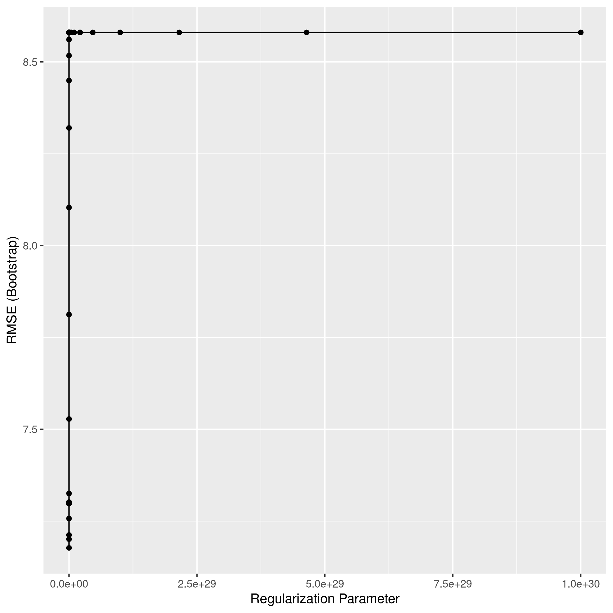
1ridgPred<-predict(ridgCol,test_set)
2ridgPred %>% postResample(obs = test_set$crim)
1##      RMSE  Rsquared       MAE
2## 6.9365371 0.3619974 2.8570012
1L1Grid <- expand.grid(alpha=1, # for lasso
2                          lambda=10^seq(from=-3,to=30,length=100))
1lassoCol<-train(crim~.,data=train_set,method="glmnet",tuneGrid = L1Grid)
1## Warning in nominalTrainWorkflow(x = x, y = y, wts = weights, info = trainInfo, :
2## There were missing values in resampled performance measures.
1lassoCol %>% summary %>% print
 1##             Length Class      Mode
 2## a0           74    -none-     numeric
 3## beta        814    dgCMatrix  S4
 4## df           74    -none-     numeric
 5## dim           2    -none-     numeric
 6## lambda       74    -none-     numeric
 7## dev.ratio    74    -none-     numeric
 8## nulldev       1    -none-     numeric
 9## npasses       1    -none-     numeric
10## jerr          1    -none-     numeric
11## offset        1    -none-     logical
12## call          5    -none-     call
13## nobs          1    -none-     numeric
14## lambdaOpt     1    -none-     numeric
15## xNames       11    -none-     character
16## problemType   1    -none-     character
17## tuneValue     2    data.frame list
18## obsLevels     1    -none-     logical
19## param         0    -none-     list
1coef(lassoCol$finalModel, lassoCol$bestTune$lambda) %>% print
 1## 12 x 1 sparse Matrix of class "dgCMatrix"
 2##                       1
 3## (Intercept)  0.86635621
 4## zn           .
 5## indus        .
 6## nox          .
 7## rm           .
 8## age          .
 9## dis          .
10## tax          0.01402174
11## ptratio      .
12## black       -0.01454496
13## lstat        0.15290845
14## medv         .
1ggplot(lassoCol)

1lassoPred<-predict(lassoCol,test_set)
2lassoPred %>% postResample(obs = test_set$crim)
1##      RMSE  Rsquared       MAE
2## 6.9630616 0.3693364 2.6767742
1rgp<-ridgCol %>% varImp %>% ggplot + ggtitle("Ridge Variable Importance")
2lsgp<-lassoCol %>% varImp %>% ggplot + ggtitle("Lasso Variable Importance")
3grid.arrange(rgp,lsgp,ncol=2,bottom="Effective Importance, scaled")
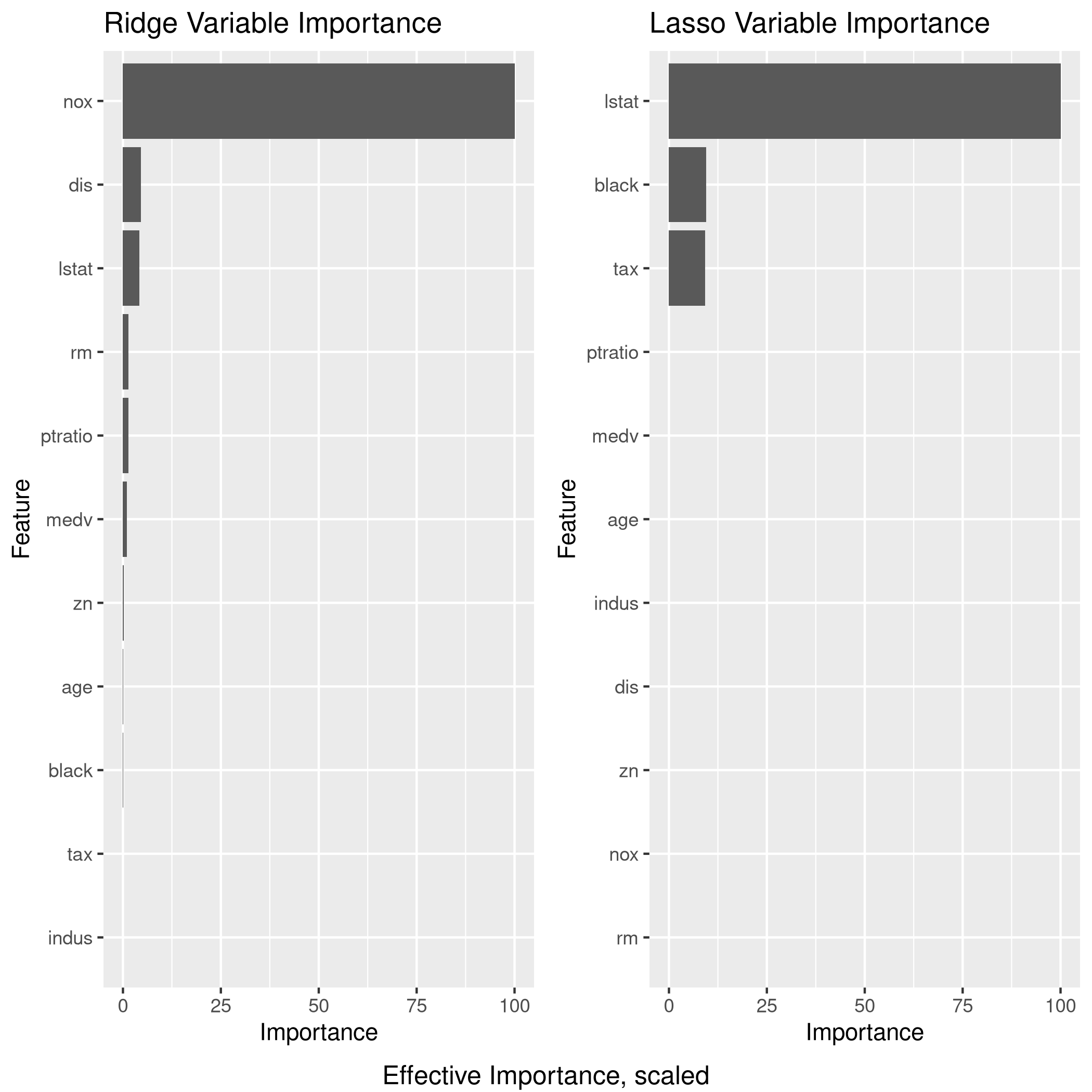
None of these models are actually any good apparently, given that we have an R² of 0.3619974 for the L2 regularization and 0.3693364 for the L1.
James, G., Witten, D., Hastie, T., & Tibshirani, R. (2013). An Introduction to Statistical Learning: with Applications in R. Berlin, Germany: Springer Science & Business Media. ↩︎
Lang et al., (2019). mlr3: A modern object-oriented machine learning framework in R. Journal of Open Source Software, 4(44), 1903, https://doi.org/10.21105/joss.01903 ↩︎
![]()