
28 minutes
Written: 2020-02-19 09:47 +0000
ISLR :: Moving Beyond Linearity
Chapter VII - Moving Beyond Linearity
All the questions are as per the ISL seventh printing of the First edition1.
Common
1libsUsed<-c("dplyr","ggplot2","tidyverse",
2            "ISLR","caret","MASS", "gridExtra",
3            "pls","latex2exp","data.table")
4invisible(lapply(libsUsed, library, character.only = TRUE))
Question 7.6 - Page 299
In this exercise, you will further analyze the Wage data set
considered throughout this chapter.
(a) Perform polynomial regression to predict wage using age. Use
cross-validation to select the optimal degree d for the polynomial.
What degree was chosen, and how does this compare to the results of
hypothesis testing using ANOVA? Make a plot of the resulting polynomial
fit to the data.
(b) Fit a step function to predict wage using age, and perform
cross-validation to choose the optimal number of cuts. Make a plot of
the fit obtained. In this exercise, we will generate simulated data, and
will then use this data to perform best subset selection.
Answer
Lets get the data.
1set.seed(1984)
2wageDat<-ISLR::Wage
3wageDat %>% str %>% print
 1## 'data.frame':    3000 obs. of  11 variables:
 2##  $ year      : int  2006 2004 2003 2003 2005 2008 2009 2008 2006 2004 ...
 3##  $ age       : int  18 24 45 43 50 54 44 30 41 52 ...
 4##  $ maritl    : Factor w/ 5 levels "1. Never Married",..: 1 1 2 2 4 2 2 1 1 2 ...
 5##  $ race      : Factor w/ 4 levels "1. White","2. Black",..: 1 1 1 3 1 1 4 3 2 1 ...
 6##  $ education : Factor w/ 5 levels "1. < HS Grad",..: 1 4 3 4 2 4 3 3 3 2 ...
 7##  $ region    : Factor w/ 9 levels "1. New England",..: 2 2 2 2 2 2 2 2 2 2 ...
 8##  $ jobclass  : Factor w/ 2 levels "1. Industrial",..: 1 2 1 2 2 2 1 2 2 2 ...
 9##  $ health    : Factor w/ 2 levels "1. <=Good","2. >=Very Good": 1 2 1 2 1 2 2 1 2 2 ...
10##  $ health_ins: Factor w/ 2 levels "1. Yes","2. No": 2 2 1 1 1 1 1 1 1 1 ...
11##  $ logwage   : num  4.32 4.26 4.88 5.04 4.32 ...
12##  $ wage      : num  75 70.5 131 154.7 75 ...
13## NULL
1wageDat %>% summary %>% print
 1##       year           age                     maritl           race
 2##  Min.   :2003   Min.   :18.00   1. Never Married: 648   1. White:2480
 3##  1st Qu.:2004   1st Qu.:33.75   2. Married      :2074   2. Black: 293
 4##  Median :2006   Median :42.00   3. Widowed      :  19   3. Asian: 190
 5##  Mean   :2006   Mean   :42.41   4. Divorced     : 204   4. Other:  37
 6##  3rd Qu.:2008   3rd Qu.:51.00   5. Separated    :  55
 7##  Max.   :2009   Max.   :80.00
 8##
 9##               education                     region               jobclass
10##  1. < HS Grad      :268   2. Middle Atlantic   :3000   1. Industrial :1544
11##  2. HS Grad        :971   1. New England       :   0   2. Information:1456
12##  3. Some College   :650   3. East North Central:   0
13##  4. College Grad   :685   4. West North Central:   0
14##  5. Advanced Degree:426   5. South Atlantic    :   0
15##                           6. East South Central:   0
16##                           (Other)              :   0
17##             health      health_ins      logwage           wage
18##  1. <=Good     : 858   1. Yes:2083   Min.   :3.000   Min.   : 20.09
19##  2. >=Very Good:2142   2. No : 917   1st Qu.:4.447   1st Qu.: 85.38
20##                                      Median :4.653   Median :104.92
21##                                      Mean   :4.654   Mean   :111.70
22##                                      3rd Qu.:4.857   3rd Qu.:128.68
23##                                      Max.   :5.763   Max.   :318.34
24##
1wageDat %>% sapply(unique) %>% sapply(length) %>% print
1##       year        age     maritl       race  education     region   jobclass
2##          7         61          5          4          5          1          2
3##     health health_ins    logwage       wage
4##          2          2        508        508
1library(boot)
1##
2## Attaching package: 'boot'
1## The following object is masked from 'package:lattice':
2##
3##     melanoma
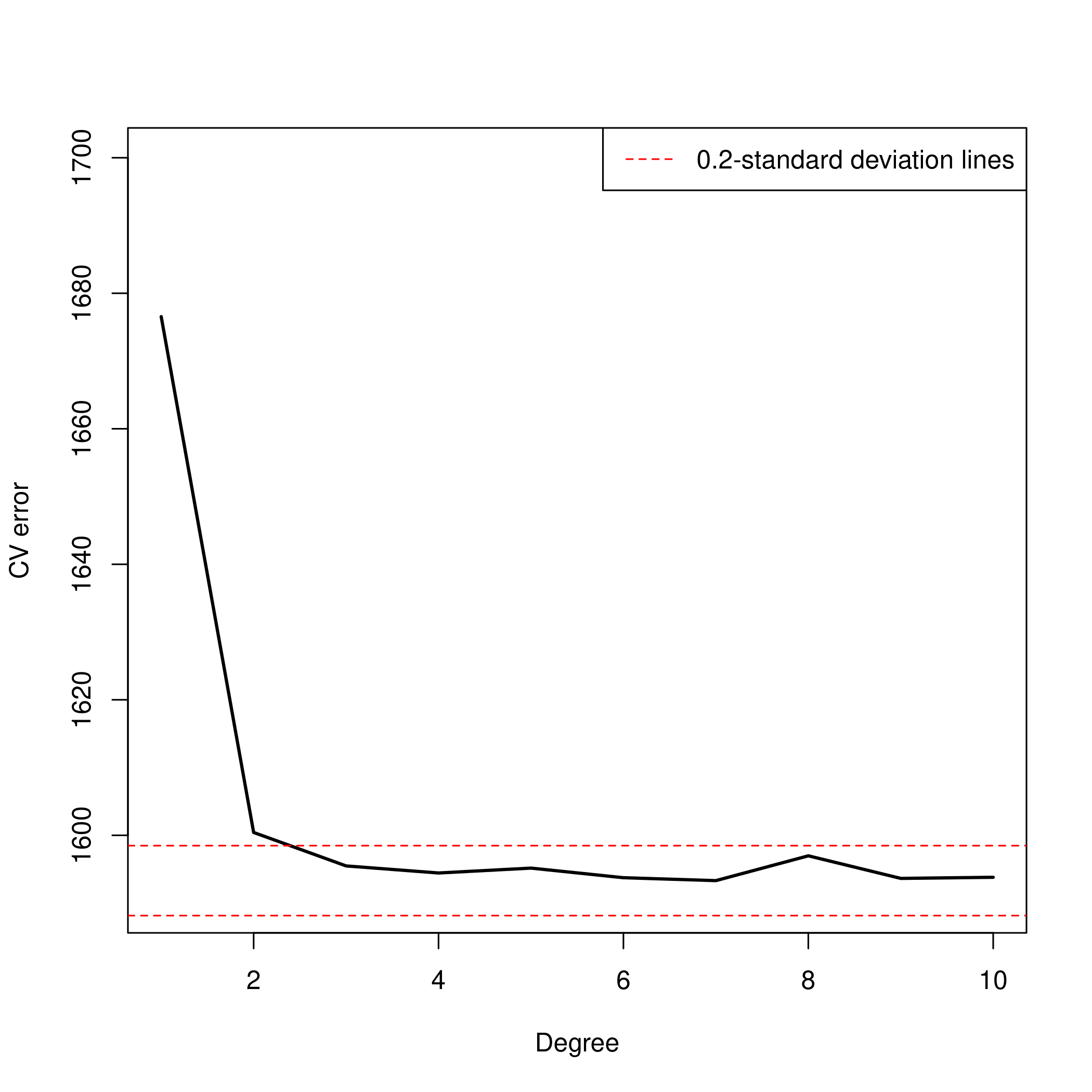
a) Polynomial regression
 1all.deltas = rep(NA, 10)
 2for (i in 1:10) {
 3  glm.fit = glm(wage~poly(age, i), data=Wage)
 4  all.deltas[i] = cv.glm(Wage, glm.fit, K=10)$delta[2]
 5}
 6plot(1:10, all.deltas, xlab="Degree", ylab="CV error", type="l", pch=20, lwd=2, ylim=c(1590, 1700))
 7min.point = min(all.deltas)
 8sd.points = sd(all.deltas)
 9abline(h=min.point + 0.2 * sd.points, col="red", lty="dashed")
10abline(h=min.point - 0.2 * sd.points, col="red", lty="dashed")
11legend("topright", "0.2-standard deviation lines", lty="dashed", col="red")
1# ANOVA
2fits=list()
3for (i in 1:10) {
4  fits[[i]]=glm(wage~poly(age,i),data=wageDat)
5}
6anova(fits[[1]],fits[[2]],fits[[3]],fits[[4]],fits[[5]],
7  fits[[6]],fits[[7]],fits[[8]],fits[[9]],fits[[10]])
 1## Analysis of Deviance Table
 2##
 3## Model  1: wage ~ poly(age, i)
 4## Model  2: wage ~ poly(age, i)
 5## Model  3: wage ~ poly(age, i)
 6## Model  4: wage ~ poly(age, i)
 7## Model  5: wage ~ poly(age, i)
 8## Model  6: wage ~ poly(age, i)
 9## Model  7: wage ~ poly(age, i)
10## Model  8: wage ~ poly(age, i)
11## Model  9: wage ~ poly(age, i)
12## Model 10: wage ~ poly(age, i)
13##    Resid. Df Resid. Dev Df Deviance
14## 1       2998    5022216
15## 2       2997    4793430  1   228786
16## 3       2996    4777674  1    15756
17## 4       2995    4771604  1     6070
18## 5       2994    4770322  1     1283
19## 6       2993    4766389  1     3932
20## 7       2992    4763834  1     2555
21## 8       2991    4763707  1      127
22## 9       2990    4756703  1     7004
23## 10      2989    4756701  1        3
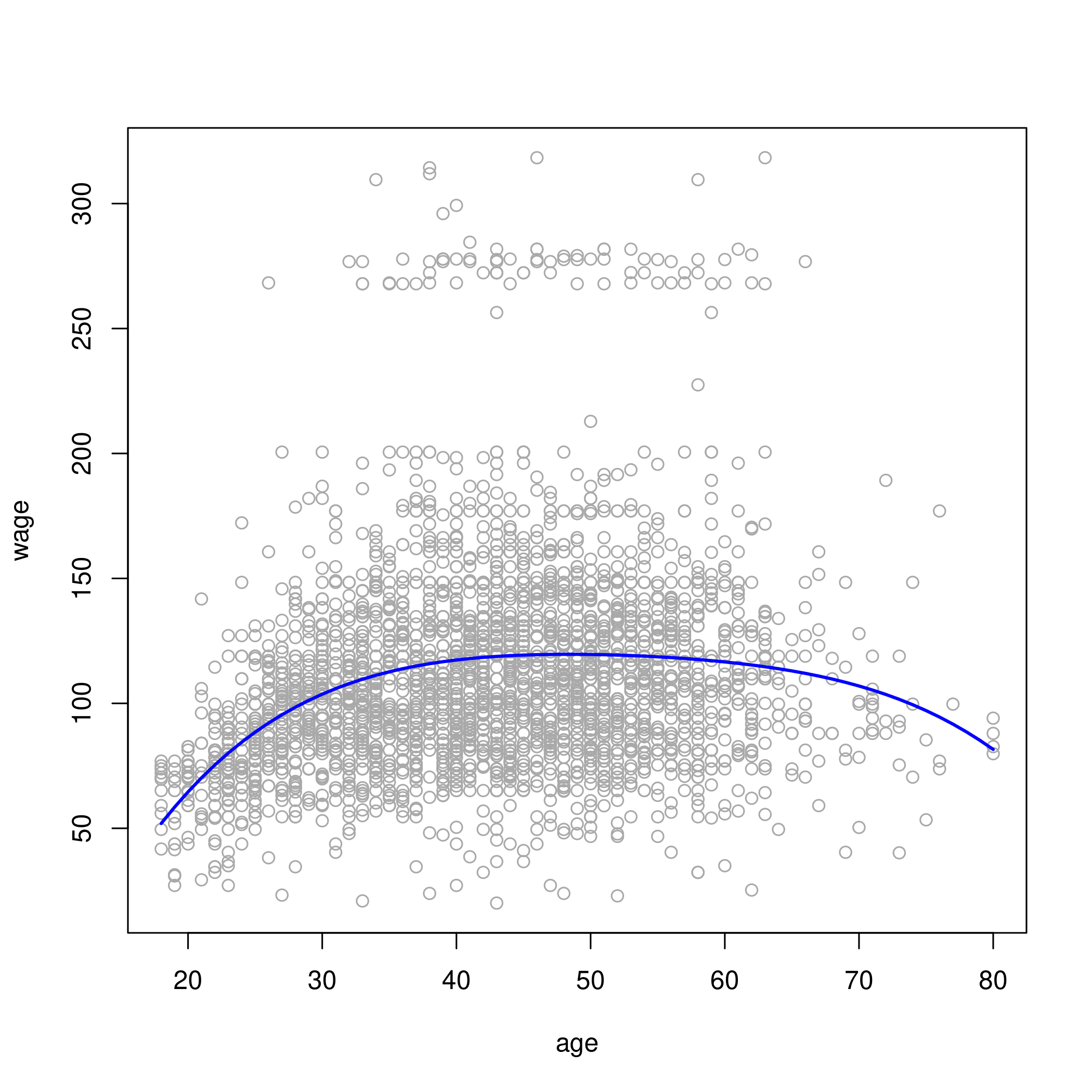
- The 4th degree looks the best at the moment
1# 3rd or 4th degrees look best based on ANOVA test
2# let's go with 4th degree fit
3plot(wage~age, data=wageDat, col="darkgrey")
4agelims = range(wageDat$age)
5age.grid = seq(from=agelims[1], to=agelims[2])
6lm.fit = lm(wage~poly(age, 4), data=wageDat)
7lm.pred = predict(lm.fit, data.frame(age=age.grid))
8lines(age.grid, lm.pred, col="blue", lwd=2)
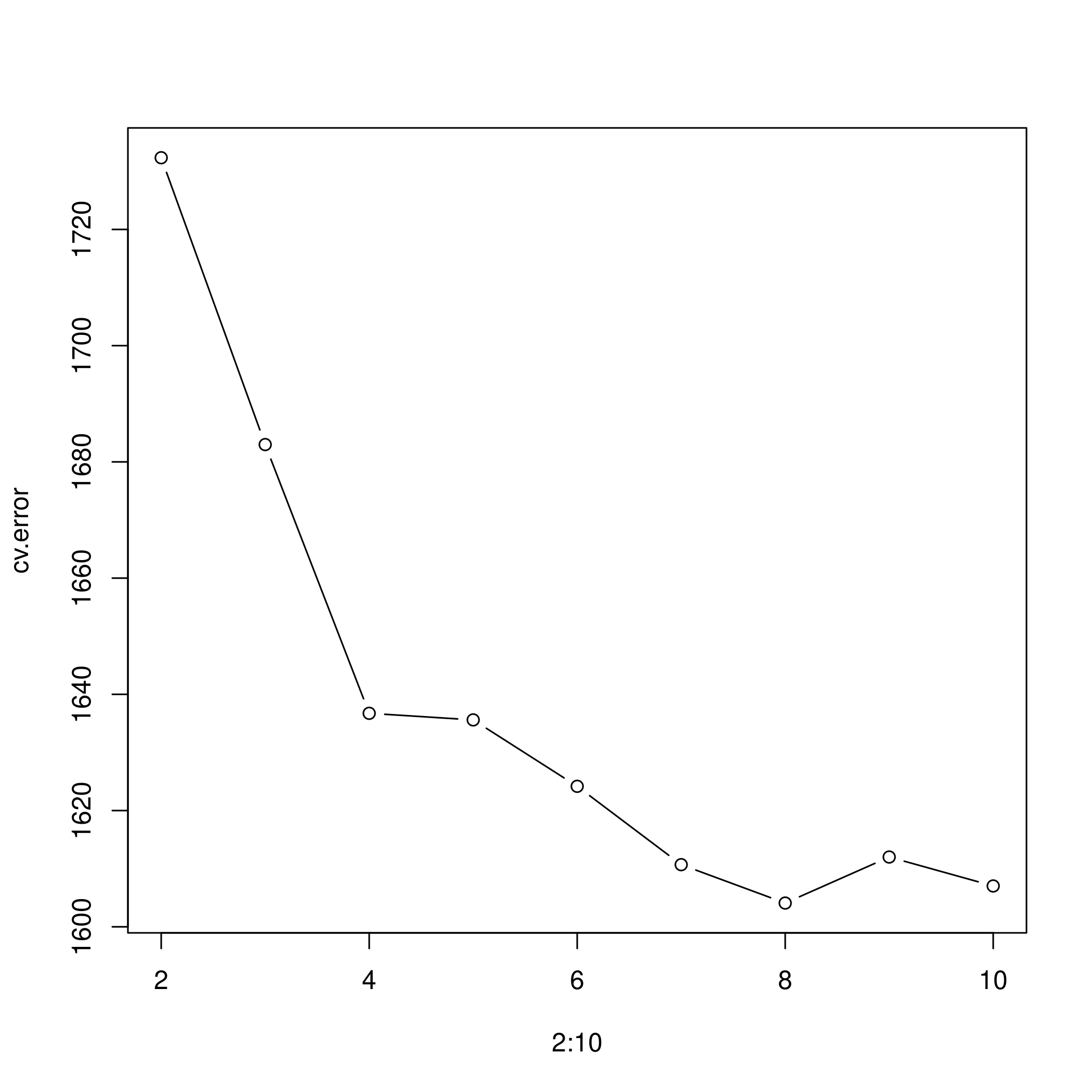
b) Step function and cross-validation
1# cross-validation
2cv.error <- rep(0,9)
3for (i in 2:10) {
4  wageDat$age.cut <- cut(wageDat$age,i)
5  glm.fit <- glm(wage~age.cut, data=wageDat)
6  cv.error[i-1] <- cv.glm(wageDat, glm.fit, K=10)$delta[1]  # [1]:std, [2]:bias-corrected
7}
8cv.error
1## [1] 1732.337 1682.978 1636.736 1635.600 1624.174 1610.688 1604.081 1612.005
2## [9] 1607.022
1cv.error
1## [1] 1732.337 1682.978 1636.736 1635.600 1624.174 1610.688 1604.081 1612.005
2## [9] 1607.022
1plot(2:10, cv.error, type="b")
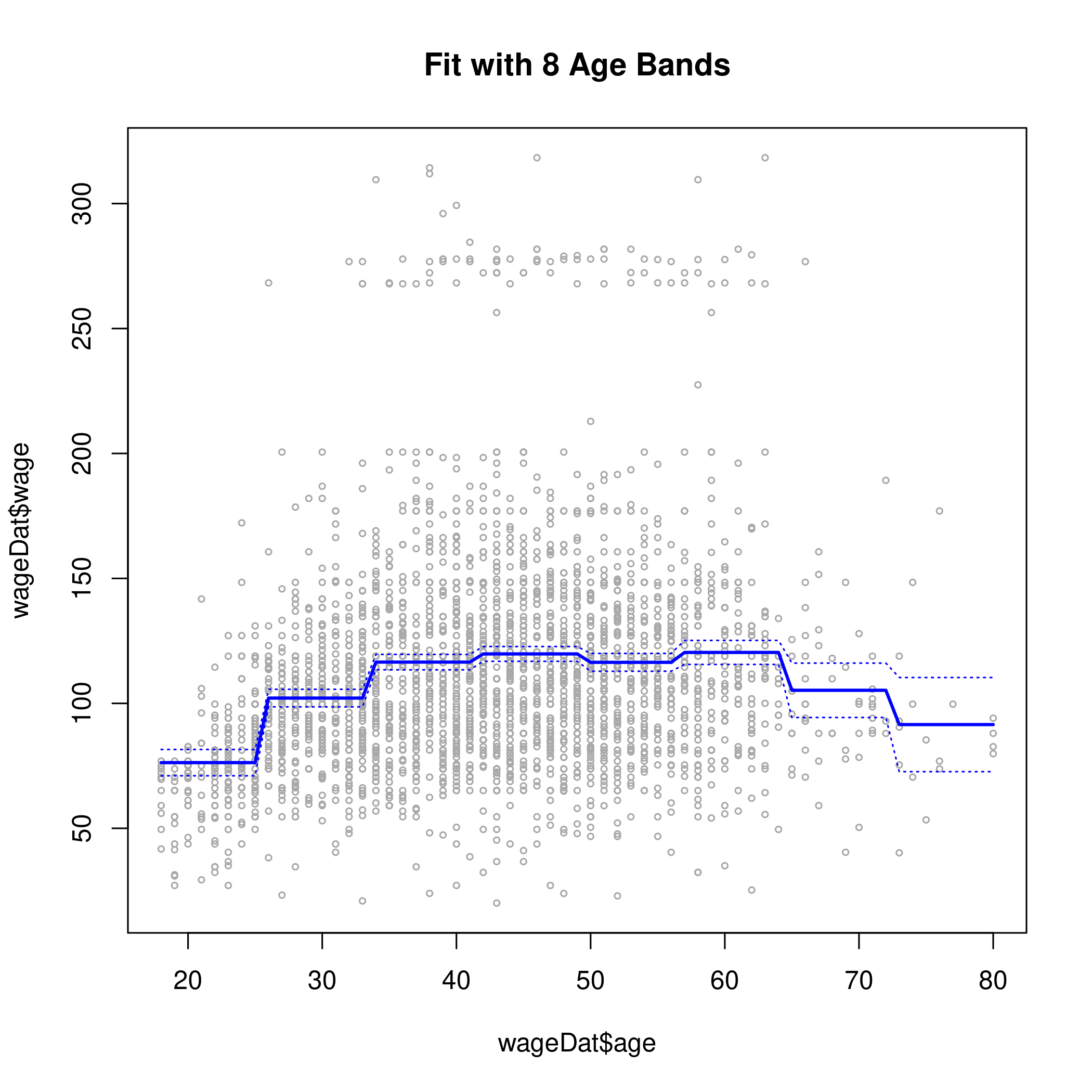
1cut.fit <- glm(wage~cut(age,8), data=wageDat)
2preds <- predict(cut.fit, newdata=list(age=age.grid), se=TRUE)
3se.bands <- preds$fit + cbind(2*preds$se.fit, -2*preds$se.fit)
4plot(wageDat$age, wageDat$wage, xlim=agelims, cex=0.5, col="darkgrey")
5title("Fit with 8 Age Bands")
6lines(age.grid, preds$fit, lwd=2, col="blue")
7matlines(age.grid, se.bands, lwd=1, col="blue", lty=3)
Question 7.8 - Page 299
Fit some of the non-linear models investigated in this chapter to the
Auto data set. Is there evidence for non-linear relationships in this
data set? Create some informative plots to justify your answer.
Answer
1autoDat<-ISLR::Auto
1autoDat %>% pivot_longer(-c(mpg,name),names_to="Params",values_to="Value") %>% ggplot(aes(x=mpg,y=Value)) +
2  geom_point() +
3  facet_wrap(~ Params, scales = "free_y")
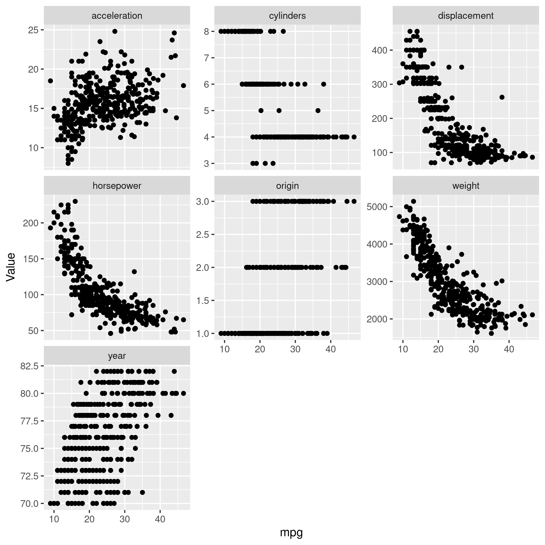
Very clearly there is a lot of non-linearity in the mpg data,
especially for acceleration, weight, displacement, horsepower.
1rss = rep(NA, 10)
2fits = list()
3for (d in 1:10) {
4    fits[[d]] = lm(mpg ~ poly(displacement, d), data = autoDat)
5    rss[d] = deviance(fits[[d]])
6}
7rss %>% print
1##  [1] 8378.822 7412.263 7392.322 7391.722 7380.838 7270.746 7089.716 6917.401
2##  [9] 6737.801 6610.190
1anova(fits[[1]],fits[[2]],fits[[3]],fits[[4]],fits[[5]],
2  fits[[6]],fits[[7]],fits[[8]],fits[[9]],fits[[10]])
 1## Analysis of Variance Table
 2##
 3## Model  1: mpg ~ poly(displacement, d)
 4## Model  2: mpg ~ poly(displacement, d)
 5## Model  3: mpg ~ poly(displacement, d)
 6## Model  4: mpg ~ poly(displacement, d)
 7## Model  5: mpg ~ poly(displacement, d)
 8## Model  6: mpg ~ poly(displacement, d)
 9## Model  7: mpg ~ poly(displacement, d)
10## Model  8: mpg ~ poly(displacement, d)
11## Model  9: mpg ~ poly(displacement, d)
12## Model 10: mpg ~ poly(displacement, d)
13##    Res.Df    RSS Df Sum of Sq       F    Pr(>F)
14## 1     390 8378.8
15## 2     389 7412.3  1    966.56 55.7108 5.756e-13 ***
16## 3     388 7392.3  1     19.94  1.1494  0.284364
17## 4     387 7391.7  1      0.60  0.0346  0.852549
18## 5     386 7380.8  1     10.88  0.6273  0.428823
19## 6     385 7270.7  1    110.09  6.3455  0.012177 *
20## 7     384 7089.7  1    181.03 10.4343  0.001344 **
21## 8     383 6917.4  1    172.31  9.9319  0.001753 **
22## 9     382 6737.8  1    179.60 10.3518  0.001404 **
23## 10    381 6610.2  1    127.61  7.3553  0.006990 **
24## ---
25## Signif. codes:  0 '***' 0.001 '**' 0.01 '*' 0.05 '.' 0.1 ' ' 1
Confirming our visual indications, we see that the second degree models work well.
1library(glmnet)
1## Loading required package: Matrix
1##
2## Attaching package: 'Matrix'
1## The following objects are masked from 'package:tidyr':
2##
3##     expand, pack, unpack
1## Loaded glmnet 3.0-2
1library(boot)
1cv.errs = rep(NA, 15)
2for (d in 1:15) {
3    fit = glm(mpg ~ poly(displacement, d), data = Auto)
4    cv.errs[d] = cv.glm(Auto, fit, K = 15)$delta[2]
5}
6which.min(cv.errs)
1## [1] 10
Strangely, we seem to have ended up with a ten variable model here.
1# Step functions
2cv.errs = rep(NA, 10)
3for (c in 2:10) {
4    Auto$dis.cut = cut(Auto$displacement, c)
5    fit = glm(mpg ~ dis.cut, data = Auto)
6    cv.errs[c] = cv.glm(Auto, fit, K = 10)$delta[2]
7}
8which.min(cv.errs) %>% print
1## [1] 9
1library(splines)
2cv.errs = rep(NA, 10)
3for (df in 3:10) {
4    fit = glm(mpg ~ ns(displacement, df = df), data = Auto)
5    cv.errs[df] = cv.glm(Auto, fit, K = 10)$delta[2]
6}
7which.min(cv.errs) %>% print
1## [1] 10
1library(gam)
1## Loading required package: foreach
1##
2## Attaching package: 'foreach'
1## The following objects are masked from 'package:purrr':
2##
3##     accumulate, when
1## Loaded gam 1.16.1
1# GAMs
2fit = gam(mpg ~ s(displacement, 4) + s(horsepower, 4), data = Auto)
1## Warning in model.matrix.default(mt, mf, contrasts): non-list contrasts argument
2## ignored
1summary(fit)
 1##
 2## Call: gam(formula = mpg ~ s(displacement, 4) + s(horsepower, 4), data = Auto)
 3## Deviance Residuals:
 4##      Min       1Q   Median       3Q      Max
 5## -11.2982  -2.1592  -0.4394   2.1247  17.0946
 6##
 7## (Dispersion Parameter for gaussian family taken to be 15.3543)
 8##
 9##     Null Deviance: 23818.99 on 391 degrees of freedom
10## Residual Deviance: 5880.697 on 382.9999 degrees of freedom
11## AIC: 2194.05
12##
13## Number of Local Scoring Iterations: 2
14##
15## Anova for Parametric Effects
16##                     Df  Sum Sq Mean Sq F value  Pr(>F)
17## s(displacement, 4)   1 15254.9 15254.9 993.524 < 2e-16 ***
18## s(horsepower, 4)     1  1038.4  1038.4  67.632 3.1e-15 ***
19## Residuals          383  5880.7    15.4
20## ---
21## Signif. codes:  0 '***' 0.001 '**' 0.01 '*' 0.05 '.' 0.1 ' ' 1
22##
23## Anova for Nonparametric Effects
24##                    Npar Df Npar F     Pr(F)
25## (Intercept)
26## s(displacement, 4)       3 13.613 1.863e-08 ***
27## s(horsepower, 4)         3 15.606 1.349e-09 ***
28## ---
29## Signif. codes:  0 '***' 0.001 '**' 0.01 '*' 0.05 '.' 0.1 ' ' 1
Question 7.9 - Pages 299-300
This question uses the variables dis (the weighted mean of distances
to five Boston employment centers) and nox (nitrogen oxides
concentration in parts per 10 million) from the Boston data. We will
treat dis as the predictor and nox as the response.
(a) Use the poly() function to fit a cubic polynomial regression to
predict nox using dis. Report the regression output, and plot the
resulting data and polynomial fits.
(b) Plot the polynomial fits for a range of different polynomial degrees (say, from 1 to 10), and report the associated residual sum of squares.
(c) Perform cross-validation or another approach to select the optimal degree for the polynomial, and explain your results.
(d) Use the bs() function to fit a regression spline to predict nox
using dis. Report the output for the fit using four degrees of
freedom. How did you choose the knots? Plot the resulting fit.
(e) Now fit a regression spline for a range of degrees of freedom, and plot the resulting fits and report the resulting RSS. Describe the results obtained.
(f) Perform cross-validation or another approach in order to select the best degrees of freedom for a regression spline on this data. Describe your results.
Answer
1boston<-MASS::Boston
2boston %>% str %>% print
 1## 'data.frame':    506 obs. of  14 variables:
 2##  $ crim   : num  0.00632 0.02731 0.02729 0.03237 0.06905 ...
 3##  $ zn     : num  18 0 0 0 0 0 12.5 12.5 12.5 12.5 ...
 4##  $ indus  : num  2.31 7.07 7.07 2.18 2.18 2.18 7.87 7.87 7.87 7.87 ...
 5##  $ chas   : int  0 0 0 0 0 0 0 0 0 0 ...
 6##  $ nox    : num  0.538 0.469 0.469 0.458 0.458 0.458 0.524 0.524 0.524 0.524 ...
 7##  $ rm     : num  6.58 6.42 7.18 7 7.15 ...
 8##  $ age    : num  65.2 78.9 61.1 45.8 54.2 58.7 66.6 96.1 100 85.9 ...
 9##  $ dis    : num  4.09 4.97 4.97 6.06 6.06 ...
10##  $ rad    : int  1 2 2 3 3 3 5 5 5 5 ...
11##  $ tax    : num  296 242 242 222 222 222 311 311 311 311 ...
12##  $ ptratio: num  15.3 17.8 17.8 18.7 18.7 18.7 15.2 15.2 15.2 15.2 ...
13##  $ black  : num  397 397 393 395 397 ...
14##  $ lstat  : num  4.98 9.14 4.03 2.94 5.33 ...
15##  $ medv   : num  24 21.6 34.7 33.4 36.2 28.7 22.9 27.1 16.5 18.9 ...
16## NULL
1boston %>% summary %>% print
 1##       crim                zn             indus            chas
 2##  Min.   : 0.00632   Min.   :  0.00   Min.   : 0.46   Min.   :0.00000
 3##  1st Qu.: 0.08204   1st Qu.:  0.00   1st Qu.: 5.19   1st Qu.:0.00000
 4##  Median : 0.25651   Median :  0.00   Median : 9.69   Median :0.00000
 5##  Mean   : 3.61352   Mean   : 11.36   Mean   :11.14   Mean   :0.06917
 6##  3rd Qu.: 3.67708   3rd Qu.: 12.50   3rd Qu.:18.10   3rd Qu.:0.00000
 7##  Max.   :88.97620   Max.   :100.00   Max.   :27.74   Max.   :1.00000
 8##       nox               rm             age              dis
 9##  Min.   :0.3850   Min.   :3.561   Min.   :  2.90   Min.   : 1.130
10##  1st Qu.:0.4490   1st Qu.:5.886   1st Qu.: 45.02   1st Qu.: 2.100
11##  Median :0.5380   Median :6.208   Median : 77.50   Median : 3.207
12##  Mean   :0.5547   Mean   :6.285   Mean   : 68.57   Mean   : 3.795
13##  3rd Qu.:0.6240   3rd Qu.:6.623   3rd Qu.: 94.08   3rd Qu.: 5.188
14##  Max.   :0.8710   Max.   :8.780   Max.   :100.00   Max.   :12.127
15##       rad              tax           ptratio          black
16##  Min.   : 1.000   Min.   :187.0   Min.   :12.60   Min.   :  0.32
17##  1st Qu.: 4.000   1st Qu.:279.0   1st Qu.:17.40   1st Qu.:375.38
18##  Median : 5.000   Median :330.0   Median :19.05   Median :391.44
19##  Mean   : 9.549   Mean   :408.2   Mean   :18.46   Mean   :356.67
20##  3rd Qu.:24.000   3rd Qu.:666.0   3rd Qu.:20.20   3rd Qu.:396.23
21##  Max.   :24.000   Max.   :711.0   Max.   :22.00   Max.   :396.90
22##      lstat            medv
23##  Min.   : 1.73   Min.   : 5.00
24##  1st Qu.: 6.95   1st Qu.:17.02
25##  Median :11.36   Median :21.20
26##  Mean   :12.65   Mean   :22.53
27##  3rd Qu.:16.95   3rd Qu.:25.00
28##  Max.   :37.97   Max.   :50.00
1boston %>% sapply(unique) %>% sapply(length) %>% print
1##    crim      zn   indus    chas     nox      rm     age     dis     rad     tax
2##     504      26      76       2      81     446     356     412       9      66
3## ptratio   black   lstat    medv
4##      46     357     455     229
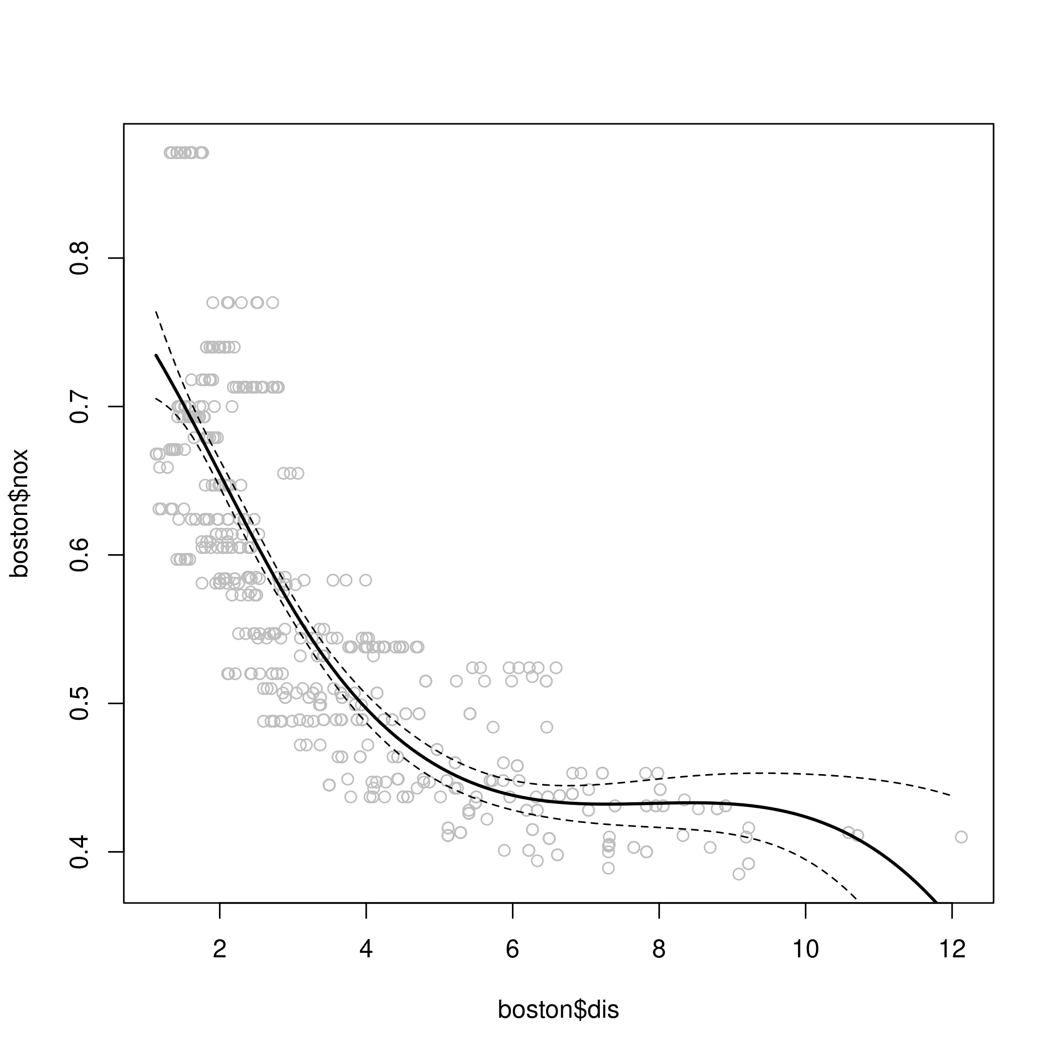
a) Polynomial
 1fit.03 <- lm(nox~poly(dis,3), data=boston)
 2dislims <- range(boston$dis)
 3dis.grid <- seq(dislims[1], dislims[2], 0.1)
 4preds <- predict(fit.03, newdata=list(dis=dis.grid), se=TRUE)
 5se.bands <- preds$fit + cbind(2*preds$se.fit, -2*preds$se.fit)
 6par(mfrow=c(1,1), mar=c(4.5,4.5,1,1), oma=c(0,0,4,0))
 7plot(boston$dis, boston$nox, xlim=dislims, cex=0.5, col="darkgrey")
 8title("Degree 3 Polynomial Fit")
 9lines(dis.grid, preds$fit, lwd=2, col="blue")
10matlines(dis.grid, se.bands, lwd=1, col="blue", lty=3)
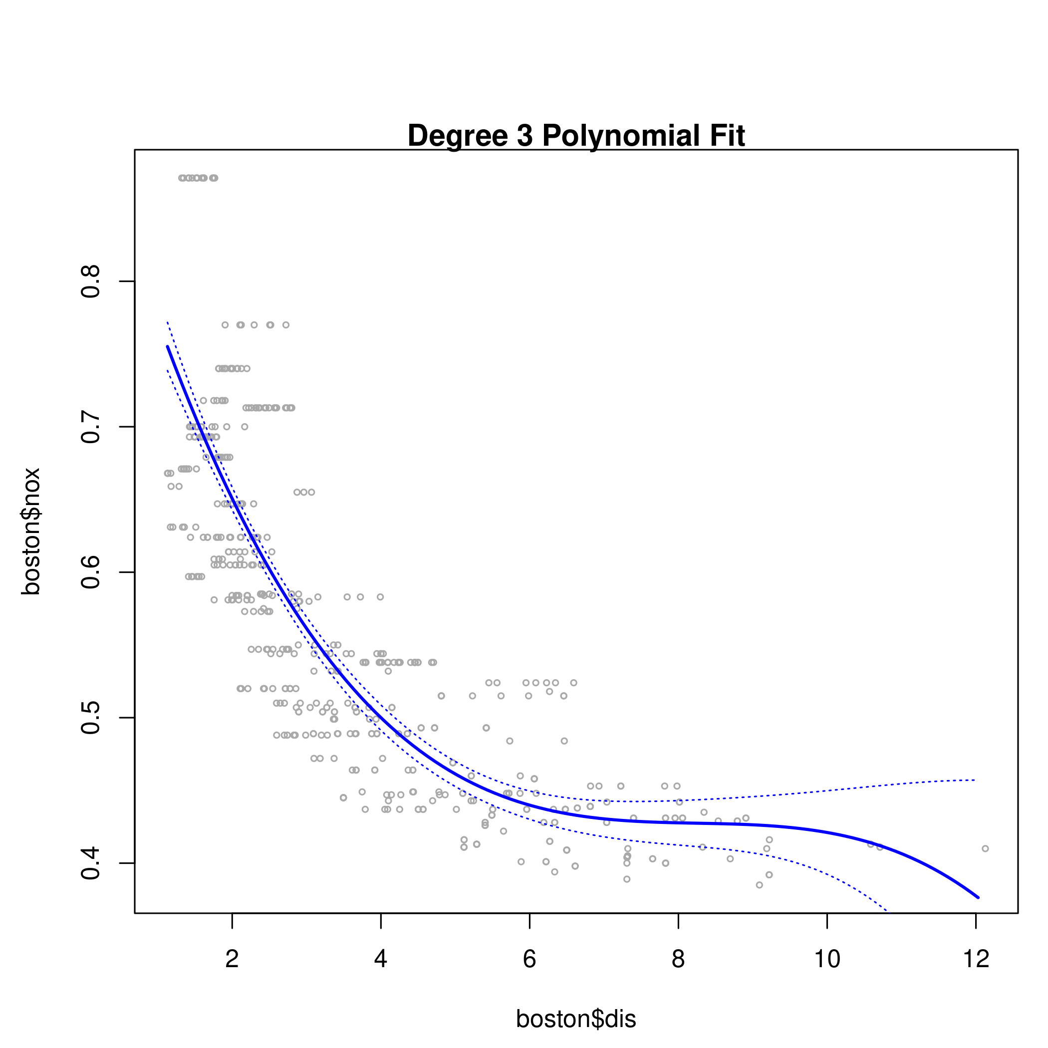
1summary(fit.03)
 1##
 2## Call:
 3## lm(formula = nox ~ poly(dis, 3), data = boston)
 4##
 5## Residuals:
 6##       Min        1Q    Median        3Q       Max
 7## -0.121130 -0.040619 -0.009738  0.023385  0.194904
 8##
 9## Coefficients:
10##                Estimate Std. Error t value Pr(>|t|)
11## (Intercept)    0.554695   0.002759 201.021  < 2e-16 ***
12## poly(dis, 3)1 -2.003096   0.062071 -32.271  < 2e-16 ***
13## poly(dis, 3)2  0.856330   0.062071  13.796  < 2e-16 ***
14## poly(dis, 3)3 -0.318049   0.062071  -5.124 4.27e-07 ***
15## ---
16## Signif. codes:  0 '***' 0.001 '**' 0.01 '*' 0.05 '.' 0.1 ' ' 1
17##
18## Residual standard error: 0.06207 on 502 degrees of freedom
19## Multiple R-squared:  0.7148, Adjusted R-squared:  0.7131
20## F-statistic: 419.3 on 3 and 502 DF,  p-value: < 2.2e-16
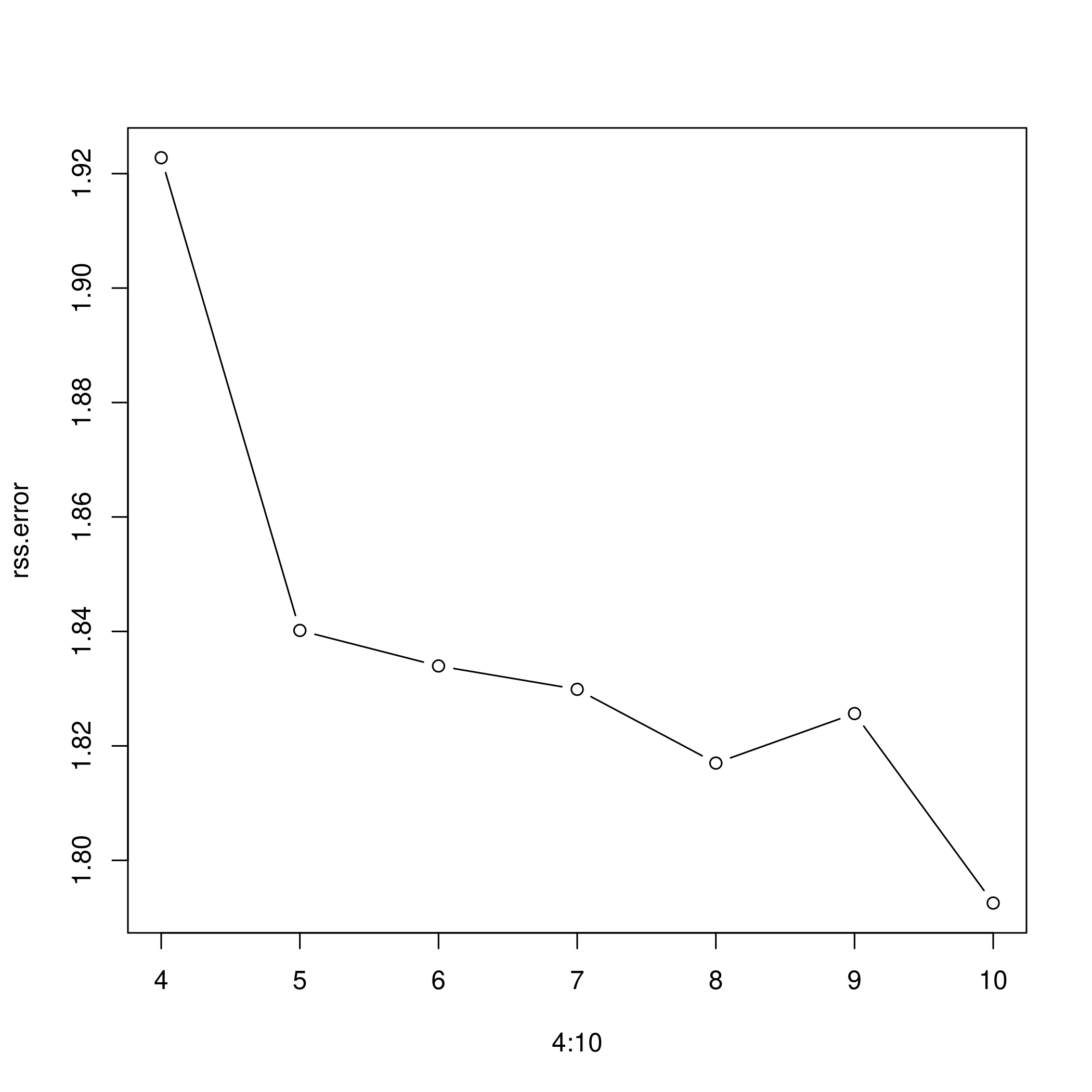
b) Multiple Polynomials
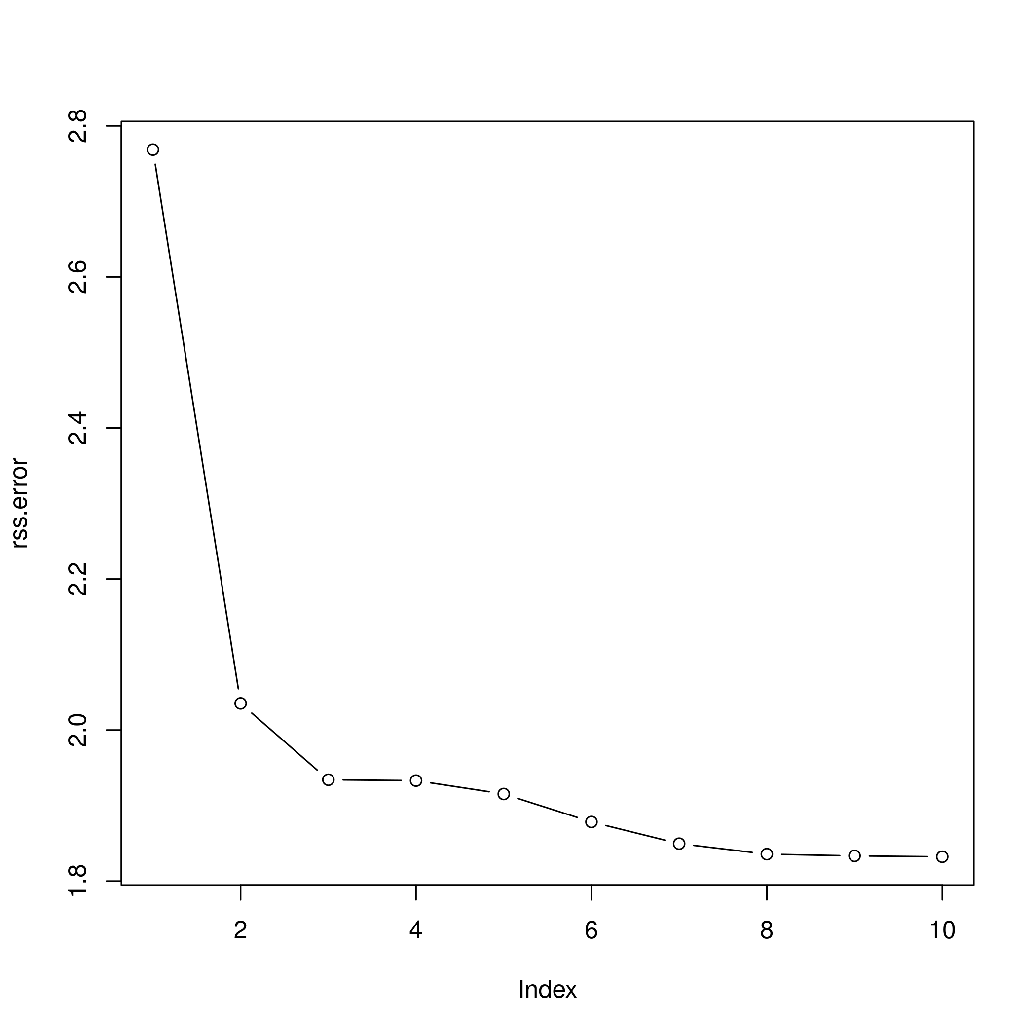
1rss.error <- rep(0,10)
2for (i in 1:10) {
3  lm.fit <- lm(nox~poly(dis,i), data=boston)
4  rss.error[i] <- sum(lm.fit$residuals^2)
5}
6rss.error
1##  [1] 2.768563 2.035262 1.934107 1.932981 1.915290 1.878257 1.849484 1.835630
2##  [9] 1.833331 1.832171
1plot(rss.error, type="b")
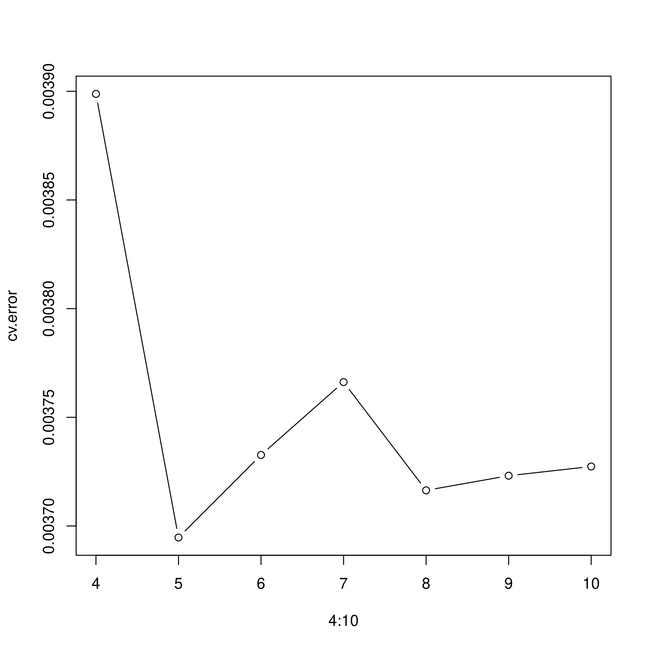
c) Cross validation and polynomial selection
1require(boot)
2set.seed(1)
3cv.error <- rep(0,10)
4for (i in 1:10) {
5  glm.fit <- glm(nox~poly(dis,i), data=boston)
6  cv.error[i] <- cv.glm(boston, glm.fit, K=10)$delta[1]  # [1]:std, [2]:bias-corrected
7}
8cv.error
1##  [1] 0.005558263 0.004085706 0.003876521 0.003863342 0.004237452 0.005686862
2##  [7] 0.010278897 0.006810868 0.033308607 0.004075599
1plot(cv.error, type="b")
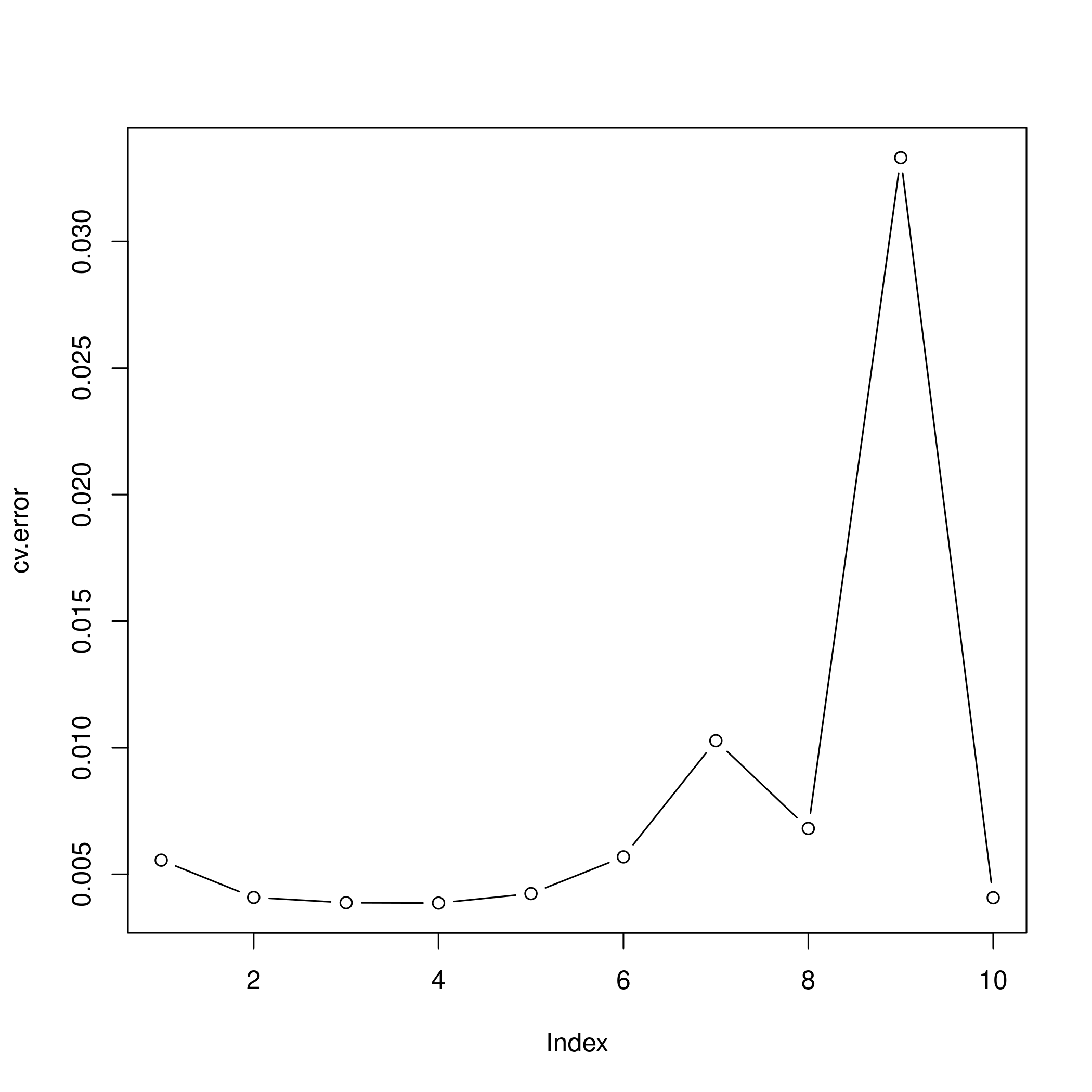
- I feel like the second degree fit would be the most reasonable, though the fourth degree seems to be doing well.
d) Regression spline
1fit.sp <- lm(nox~bs(dis, df=4), data=boston)
2pred <- predict(fit.sp, newdata=list(dis=dis.grid), se=T)
3plot(boston$dis, boston$nox, col="gray")
4lines(dis.grid, pred$fit, lwd=2)
5lines(dis.grid, pred$fit+2*pred$se, lty="dashed")
6lines(dis.grid, pred$fit-2*pred$se, lty="dashed")
1# set df to select knots at uniform quantiles of `dis`
2attr(bs(boston$dis,df=4),"knots")  # only 1 knot at 50th percentile
1##     50%
2## 3.20745
e) Range of regression splines
1rss.error <- rep(0,7)
2for (i in 4:10) {
3  fit.sp <- lm(nox~bs(dis, df=i), data=boston)
4  rss.error[i-3] <- sum(fit.sp$residuals^2)
5}
6rss.error
1## [1] 1.922775 1.840173 1.833966 1.829884 1.816995 1.825653 1.792535
1plot(4:10, rss.error, type="b")
- As the model gains more degrees of freedom, it tends to over fit to the training data better
f) Cross validation for best spline
1cv.error <- rep(0,7)
2for (i in 4:10) {
3  glm.fit <- glm(nox~bs(dis, df=i), data=boston)
4  cv.error[i-3] <- cv.glm(boston, glm.fit, K=10)$delta[1]
5}
1## Warning in bs(dis, degree = 3L, knots = c(`50%` = 3.1523), Boundary.knots =
2## c(1.1296, : some 'x' values beyond boundary knots may cause ill-conditioned
3## bases
4
5## Warning in bs(dis, degree = 3L, knots = c(`50%` = 3.1523), Boundary.knots =
6## c(1.1296, : some 'x' values beyond boundary knots may cause ill-conditioned
7## bases
1## Warning in bs(dis, degree = 3L, knots = c(`50%` = 3.2157), Boundary.knots =
2## c(1.137, : some 'x' values beyond boundary knots may cause ill-conditioned bases
3
4## Warning in bs(dis, degree = 3L, knots = c(`50%` = 3.2157), Boundary.knots =
5## c(1.137, : some 'x' values beyond boundary knots may cause ill-conditioned bases
1## Warning in bs(dis, degree = 3L, knots = c(`33.33333%` = 2.35953333333333, : some
2## 'x' values beyond boundary knots may cause ill-conditioned bases
3
4## Warning in bs(dis, degree = 3L, knots = c(`33.33333%` = 2.35953333333333, : some
5## 'x' values beyond boundary knots may cause ill-conditioned bases
1## Warning in bs(dis, degree = 3L, knots = c(`33.33333%` = 2.38403333333333, : some
2## 'x' values beyond boundary knots may cause ill-conditioned bases
3
4## Warning in bs(dis, degree = 3L, knots = c(`33.33333%` = 2.38403333333333, : some
5## 'x' values beyond boundary knots may cause ill-conditioned bases
1## Warning in bs(dis, degree = 3L, knots = c(`25%` = 2.07945, `50%` = 3.1323, :
2## some 'x' values beyond boundary knots may cause ill-conditioned bases
3
4## Warning in bs(dis, degree = 3L, knots = c(`25%` = 2.07945, `50%` = 3.1323, :
5## some 'x' values beyond boundary knots may cause ill-conditioned bases
1## Warning in bs(dis, degree = 3L, knots = c(`25%` = 2.1103, `50%` = 3.2797, : some
2## 'x' values beyond boundary knots may cause ill-conditioned bases
3
4## Warning in bs(dis, degree = 3L, knots = c(`25%` = 2.1103, `50%` = 3.2797, : some
5## 'x' values beyond boundary knots may cause ill-conditioned bases
1## Warning in bs(dis, degree = 3L, knots = c(`20%` = 1.9682, `40%` = 2.7147, : some
2## 'x' values beyond boundary knots may cause ill-conditioned bases
3
4## Warning in bs(dis, degree = 3L, knots = c(`20%` = 1.9682, `40%` = 2.7147, : some
5## 'x' values beyond boundary knots may cause ill-conditioned bases
1## Warning in bs(dis, degree = 3L, knots = c(`20%` = 1.95434, `40%` = 2.59666, :
2## some 'x' values beyond boundary knots may cause ill-conditioned bases
3
4## Warning in bs(dis, degree = 3L, knots = c(`20%` = 1.95434, `40%` = 2.59666, :
5## some 'x' values beyond boundary knots may cause ill-conditioned bases
1## Warning in bs(dis, degree = 3L, knots = c(`16.66667%` = 1.82203333333333, : some
2## 'x' values beyond boundary knots may cause ill-conditioned bases
3
4## Warning in bs(dis, degree = 3L, knots = c(`16.66667%` = 1.82203333333333, : some
5## 'x' values beyond boundary knots may cause ill-conditioned bases
1## Warning in bs(dis, degree = 3L, knots = c(`16.66667%` = 1.8226, `33.33333%` =
2## 2.3817, : some 'x' values beyond boundary knots may cause ill-conditioned bases
3
4## Warning in bs(dis, degree = 3L, knots = c(`16.66667%` = 1.8226, `33.33333%` =
5## 2.3817, : some 'x' values beyond boundary knots may cause ill-conditioned bases
1## Warning in bs(dis, degree = 3L, knots = c(`14.28571%` = 1.7936, `28.57143%`
2## = 2.16972857142857, : some 'x' values beyond boundary knots may cause ill-
3## conditioned bases
4
5## Warning in bs(dis, degree = 3L, knots = c(`14.28571%` = 1.7936, `28.57143%`
6## = 2.16972857142857, : some 'x' values beyond boundary knots may cause ill-
7## conditioned bases
1## Warning in bs(dis, degree = 3L, knots = c(`12.5%` = 1.754625, `25%` = 2.10215, :
2## some 'x' values beyond boundary knots may cause ill-conditioned bases
3
4## Warning in bs(dis, degree = 3L, knots = c(`12.5%` = 1.754625, `25%` = 2.10215, :
5## some 'x' values beyond boundary knots may cause ill-conditioned bases
1## Warning in bs(dis, degree = 3L, knots = c(`12.5%` = 1.751575, `25%` = 2.08755, :
2## some 'x' values beyond boundary knots may cause ill-conditioned bases
3
4## Warning in bs(dis, degree = 3L, knots = c(`12.5%` = 1.751575, `25%` = 2.08755, :
5## some 'x' values beyond boundary knots may cause ill-conditioned bases
1cv.error
1## [1] 0.003898810 0.003694675 0.003732665 0.003766202 0.003716389 0.003723126
2## [7] 0.003727358
1plot(4:10, cv.error, type="b")
- A fifth degree polynomial is clearly indicated
Question 10 - Page 300
This question relates to the College data set.
(a) Split the data into a training set and a test set. Using out-of-state tuition as the response and the other variables as the predictors, perform forward stepwise selection on the training set in order to identify a satisfactory model that uses just a subset of the predictors.
(b) Fit a GAM on the training data, using out-of-state tuition as the response and the features selected in the previous step as the predictors. Plot the results, and explain your findings.
(c) Evaluate the model obtained on the test set, and explain the results obtained.
(d) For which variables, if any, is there evidence of a non-linear relationship with the response?
Answer
1colDat<-ISLR::College
2colDat %>% str %>% print
 1## 'data.frame':    777 obs. of  18 variables:
 2##  $ Private    : Factor w/ 2 levels "No","Yes": 2 2 2 2 2 2 2 2 2 2 ...
 3##  $ Apps       : num  1660 2186 1428 417 193 ...
 4##  $ Accept     : num  1232 1924 1097 349 146 ...
 5##  $ Enroll     : num  721 512 336 137 55 158 103 489 227 172 ...
 6##  $ Top10perc  : num  23 16 22 60 16 38 17 37 30 21 ...
 7##  $ Top25perc  : num  52 29 50 89 44 62 45 68 63 44 ...
 8##  $ F.Undergrad: num  2885 2683 1036 510 249 ...
 9##  $ P.Undergrad: num  537 1227 99 63 869 ...
10##  $ Outstate   : num  7440 12280 11250 12960 7560 ...
11##  $ Room.Board : num  3300 6450 3750 5450 4120 ...
12##  $ Books      : num  450 750 400 450 800 500 500 450 300 660 ...
13##  $ Personal   : num  2200 1500 1165 875 1500 ...
14##  $ PhD        : num  70 29 53 92 76 67 90 89 79 40 ...
15##  $ Terminal   : num  78 30 66 97 72 73 93 100 84 41 ...
16##  $ S.F.Ratio  : num  18.1 12.2 12.9 7.7 11.9 9.4 11.5 13.7 11.3 11.5 ...
17##  $ perc.alumni: num  12 16 30 37 2 11 26 37 23 15 ...
18##  $ Expend     : num  7041 10527 8735 19016 10922 ...
19##  $ Grad.Rate  : num  60 56 54 59 15 55 63 73 80 52 ...
20## NULL
1colDat %>% summary %>% print
 1##  Private        Apps           Accept          Enroll       Top10perc
 2##  No :212   Min.   :   81   Min.   :   72   Min.   :  35   Min.   : 1.00
 3##  Yes:565   1st Qu.:  776   1st Qu.:  604   1st Qu.: 242   1st Qu.:15.00
 4##            Median : 1558   Median : 1110   Median : 434   Median :23.00
 5##            Mean   : 3002   Mean   : 2019   Mean   : 780   Mean   :27.56
 6##            3rd Qu.: 3624   3rd Qu.: 2424   3rd Qu.: 902   3rd Qu.:35.00
 7##            Max.   :48094   Max.   :26330   Max.   :6392   Max.   :96.00
 8##    Top25perc      F.Undergrad     P.Undergrad         Outstate
 9##  Min.   :  9.0   Min.   :  139   Min.   :    1.0   Min.   : 2340
10##  1st Qu.: 41.0   1st Qu.:  992   1st Qu.:   95.0   1st Qu.: 7320
11##  Median : 54.0   Median : 1707   Median :  353.0   Median : 9990
12##  Mean   : 55.8   Mean   : 3700   Mean   :  855.3   Mean   :10441
13##  3rd Qu.: 69.0   3rd Qu.: 4005   3rd Qu.:  967.0   3rd Qu.:12925
14##  Max.   :100.0   Max.   :31643   Max.   :21836.0   Max.   :21700
15##    Room.Board       Books           Personal         PhD
16##  Min.   :1780   Min.   :  96.0   Min.   : 250   Min.   :  8.00
17##  1st Qu.:3597   1st Qu.: 470.0   1st Qu.: 850   1st Qu.: 62.00
18##  Median :4200   Median : 500.0   Median :1200   Median : 75.00
19##  Mean   :4358   Mean   : 549.4   Mean   :1341   Mean   : 72.66
20##  3rd Qu.:5050   3rd Qu.: 600.0   3rd Qu.:1700   3rd Qu.: 85.00
21##  Max.   :8124   Max.   :2340.0   Max.   :6800   Max.   :103.00
22##     Terminal       S.F.Ratio      perc.alumni        Expend
23##  Min.   : 24.0   Min.   : 2.50   Min.   : 0.00   Min.   : 3186
24##  1st Qu.: 71.0   1st Qu.:11.50   1st Qu.:13.00   1st Qu.: 6751
25##  Median : 82.0   Median :13.60   Median :21.00   Median : 8377
26##  Mean   : 79.7   Mean   :14.09   Mean   :22.74   Mean   : 9660
27##  3rd Qu.: 92.0   3rd Qu.:16.50   3rd Qu.:31.00   3rd Qu.:10830
28##  Max.   :100.0   Max.   :39.80   Max.   :64.00   Max.   :56233
29##    Grad.Rate
30##  Min.   : 10.00
31##  1st Qu.: 53.00
32##  Median : 65.00
33##  Mean   : 65.46
34##  3rd Qu.: 78.00
35##  Max.   :118.00
1colDat %>% sapply(unique) %>% sapply(length) %>% print
1##     Private        Apps      Accept      Enroll   Top10perc   Top25perc
2##           2         711         693         581          82          89
3## F.Undergrad P.Undergrad    Outstate  Room.Board       Books    Personal
4##         714         566         640         553         122         294
5##         PhD    Terminal   S.F.Ratio perc.alumni      Expend   Grad.Rate
6##          78          65         173          61         744          81
 1plotLEAP=function(leapObj){
 2  par(mfrow = c(2,2))
 3  bar2=which.max(leapObj$adjr2)
 4  bbic=which.min(leapObj$bic)
 5  bcp=which.min(leapObj$cp)
 6  plot(leapObj$rss,xlab="Number of variables",ylab="RSS",type="b")
 7  plot(leapObj$adjr2,xlab="Number of variables",ylab=TeX("Adjusted R^2"),type="b")
 8  points(bar2,leapObj$adjr2[bar2],col="green",cex=2,pch=20)
 9  plot(leapObj$bic,xlab="Number of variables",ylab=TeX("BIC"),type="b")
10  points(bbic,leapObj$bic[bbic],col="blue",cex=2,pch=20)
11  plot(leapObj$cp,xlab="Number of variables",ylab=TeX("C_p"),type="b")
12  points(bcp,leapObj$cp[bcp],col="red",cex=2,pch=20)
13}
a) Train test
1train_ind = sample(colDat %>% nrow,100)
2test_ind = setdiff(seq_len(colDat %>% nrow), train_ind)
Best subset selection
1train_set<-colDat[train_ind,]
2test_set<-colDat[-train_ind,]
1library(leaps)
1modelFit<-regsubsets(Outstate~.,data=colDat,nvmax=20)
2modelFit %>% summary %>% print
 1## Subset selection object
 2## Call: regsubsets.formula(Outstate ~ ., data = colDat, nvmax = 20)
 3## 17 Variables  (and intercept)
 4##             Forced in Forced out
 5## PrivateYes      FALSE      FALSE
 6## Apps            FALSE      FALSE
 7## Accept          FALSE      FALSE
 8## Enroll          FALSE      FALSE
 9## Top10perc       FALSE      FALSE
10## Top25perc       FALSE      FALSE
11## F.Undergrad     FALSE      FALSE
12## P.Undergrad     FALSE      FALSE
13## Room.Board      FALSE      FALSE
14## Books           FALSE      FALSE
15## Personal        FALSE      FALSE
16## PhD             FALSE      FALSE
17## Terminal        FALSE      FALSE
18## S.F.Ratio       FALSE      FALSE
19## perc.alumni     FALSE      FALSE
20## Expend          FALSE      FALSE
21## Grad.Rate       FALSE      FALSE
22## 1 subsets of each size up to 17
23## Selection Algorithm: exhaustive
24##           PrivateYes Apps Accept Enroll Top10perc Top25perc F.Undergrad
25## 1  ( 1 )  " "        " "  " "    " "    " "       " "       " "
26## 2  ( 1 )  "*"        " "  " "    " "    " "       " "       " "
27## 3  ( 1 )  "*"        " "  " "    " "    " "       " "       " "
28## 4  ( 1 )  "*"        " "  " "    " "    " "       " "       " "
29## 5  ( 1 )  "*"        " "  " "    " "    " "       " "       " "
30## 6  ( 1 )  "*"        " "  " "    " "    " "       " "       " "
31## 7  ( 1 )  "*"        " "  " "    " "    " "       " "       " "
32## 8  ( 1 )  "*"        " "  "*"    " "    " "       " "       "*"
33## 9  ( 1 )  "*"        "*"  "*"    " "    " "       " "       "*"
34## 10  ( 1 ) "*"        "*"  "*"    " "    "*"       " "       "*"
35## 11  ( 1 ) "*"        "*"  "*"    " "    "*"       " "       "*"
36## 12  ( 1 ) "*"        "*"  "*"    " "    "*"       " "       "*"
37## 13  ( 1 ) "*"        "*"  "*"    "*"    "*"       " "       "*"
38## 14  ( 1 ) "*"        "*"  "*"    "*"    "*"       " "       "*"
39## 15  ( 1 ) "*"        "*"  "*"    "*"    "*"       " "       "*"
40## 16  ( 1 ) "*"        "*"  "*"    "*"    "*"       "*"       "*"
41## 17  ( 1 ) "*"        "*"  "*"    "*"    "*"       "*"       "*"
42##           P.Undergrad Room.Board Books Personal PhD Terminal S.F.Ratio
43## 1  ( 1 )  " "         " "        " "   " "      " " " "      " "
44## 2  ( 1 )  " "         " "        " "   " "      " " " "      " "
45## 3  ( 1 )  " "         "*"        " "   " "      " " " "      " "
46## 4  ( 1 )  " "         "*"        " "   " "      " " " "      " "
47## 5  ( 1 )  " "         "*"        " "   " "      "*" " "      " "
48## 6  ( 1 )  " "         "*"        " "   " "      " " "*"      " "
49## 7  ( 1 )  " "         "*"        " "   "*"      " " "*"      " "
50## 8  ( 1 )  " "         "*"        " "   " "      " " "*"      " "
51## 9  ( 1 )  " "         "*"        " "   " "      " " "*"      " "
52## 10  ( 1 ) " "         "*"        " "   " "      " " "*"      " "
53## 11  ( 1 ) " "         "*"        " "   "*"      " " "*"      " "
54## 12  ( 1 ) " "         "*"        " "   "*"      " " "*"      "*"
55## 13  ( 1 ) " "         "*"        " "   "*"      " " "*"      "*"
56## 14  ( 1 ) " "         "*"        " "   "*"      "*" "*"      "*"
57## 15  ( 1 ) " "         "*"        "*"   "*"      "*" "*"      "*"
58## 16  ( 1 ) " "         "*"        "*"   "*"      "*" "*"      "*"
59## 17  ( 1 ) "*"         "*"        "*"   "*"      "*" "*"      "*"
60##           perc.alumni Expend Grad.Rate
61## 1  ( 1 )  " "         "*"    " "
62## 2  ( 1 )  " "         "*"    " "
63## 3  ( 1 )  " "         "*"    " "
64## 4  ( 1 )  "*"         "*"    " "
65## 5  ( 1 )  "*"         "*"    " "
66## 6  ( 1 )  "*"         "*"    "*"
67## 7  ( 1 )  "*"         "*"    "*"
68## 8  ( 1 )  "*"         "*"    "*"
69## 9  ( 1 )  "*"         "*"    "*"
70## 10  ( 1 ) "*"         "*"    "*"
71## 11  ( 1 ) "*"         "*"    "*"
72## 12  ( 1 ) "*"         "*"    "*"
73## 13  ( 1 ) "*"         "*"    "*"
74## 14  ( 1 ) "*"         "*"    "*"
75## 15  ( 1 ) "*"         "*"    "*"
76## 16  ( 1 ) "*"         "*"    "*"
77## 17  ( 1 ) "*"         "*"    "*"
We might want to take a look at these.
1par(mfrow=c(2,2))
2plot(modelFit)
3plot(modelFit,scale='Cp')
4plot(modelFit,scale='r2')
5plot(modelFit,scale='adjr2')
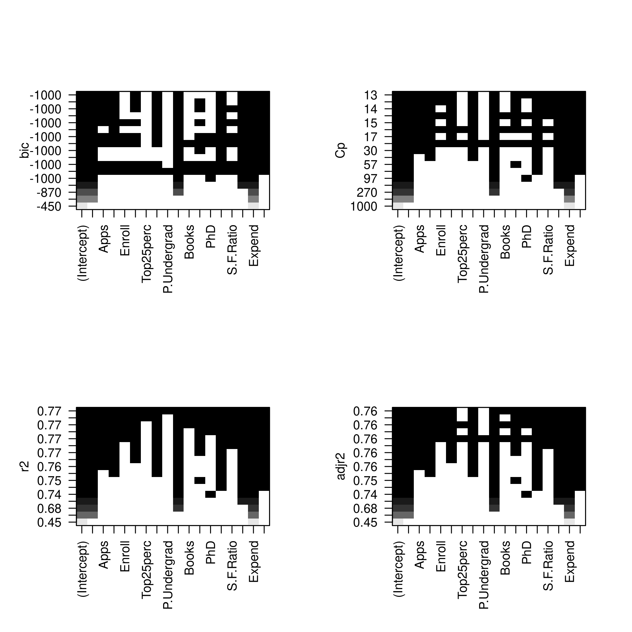
1plotLEAP(modelFit %>% summary)
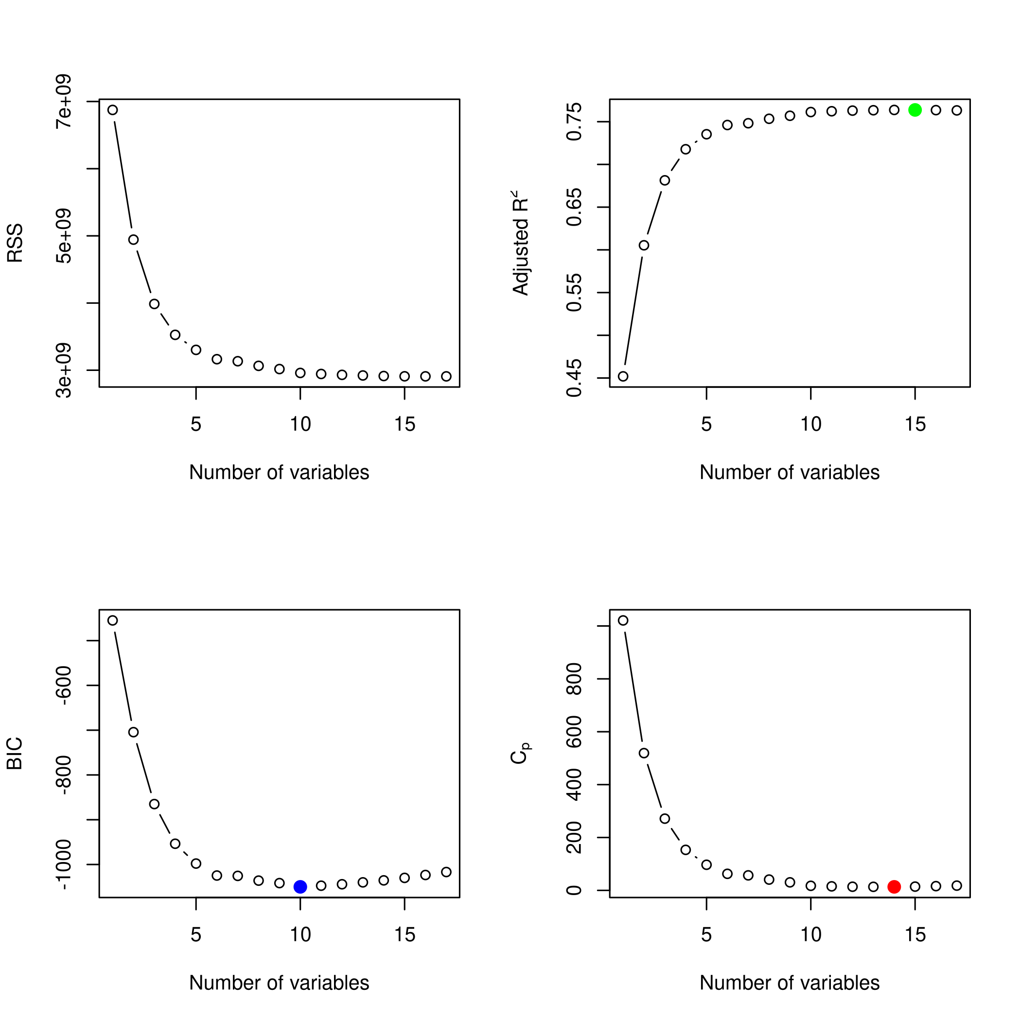
- So we like 14 variables, namely
1coefficients(modelFit,id=14) %>% print
1##   (Intercept)    PrivateYes          Apps        Accept        Enroll
2## -1.817040e+03  2.256946e+03 -2.999022e-01  8.023519e-01 -5.372545e-01
3##     Top10perc   F.Undergrad    Room.Board      Personal           PhD
4##  2.365529e+01 -9.569936e-02  8.741819e-01 -2.478418e-01  1.269506e+01
5##      Terminal     S.F.Ratio   perc.alumni        Expend     Grad.Rate
6##  2.297296e+01 -4.700560e+01  4.195006e+01  2.003912e-01  2.383197e+01
- But five seems like a better bet.
1coefficients(modelFit,id=5)
1##   (Intercept)    PrivateYes    Room.Board           PhD   perc.alumni
2## -2864.6325619  2936.7416766     1.0677573    40.5334088    61.3147684
3##        Expend
4##     0.2253945
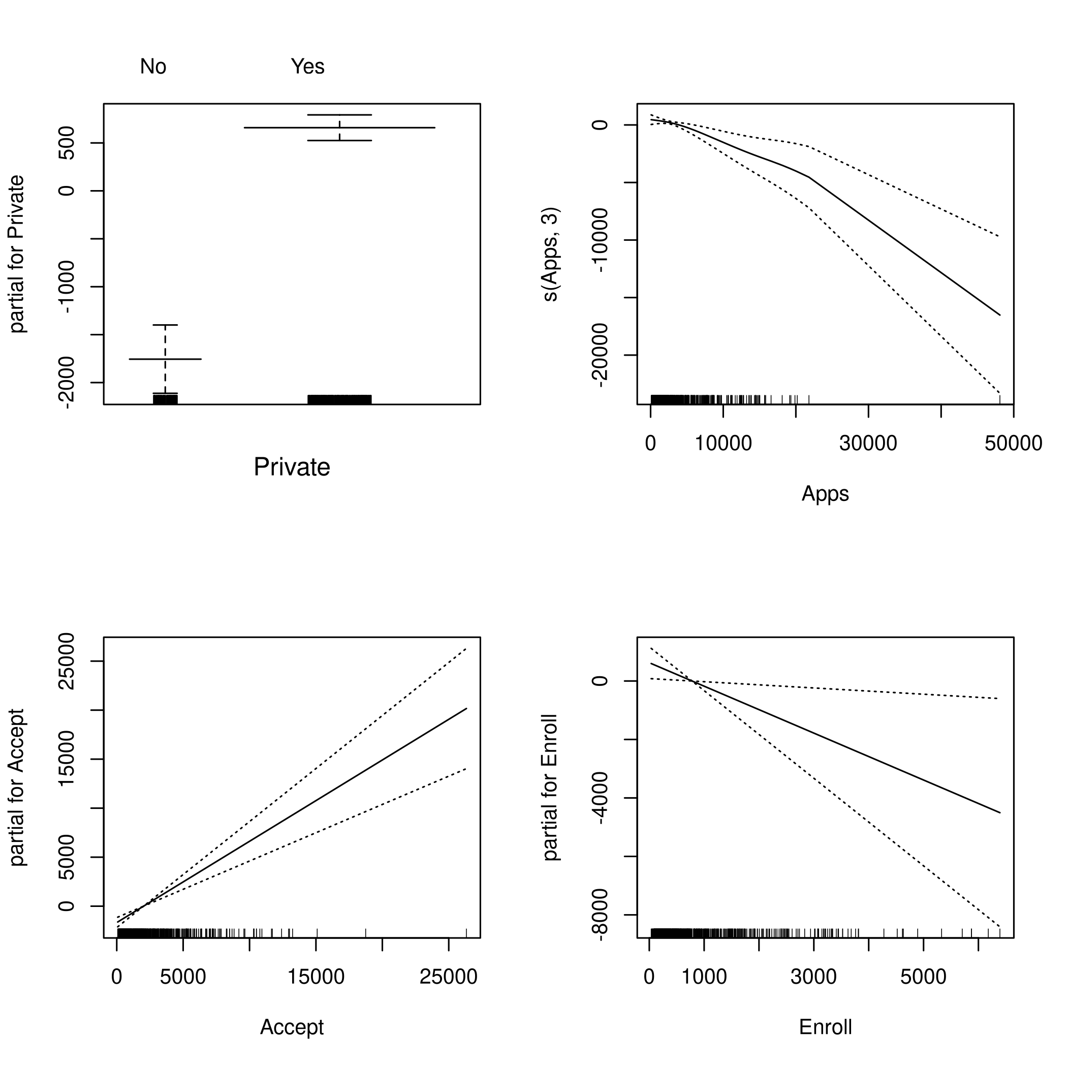
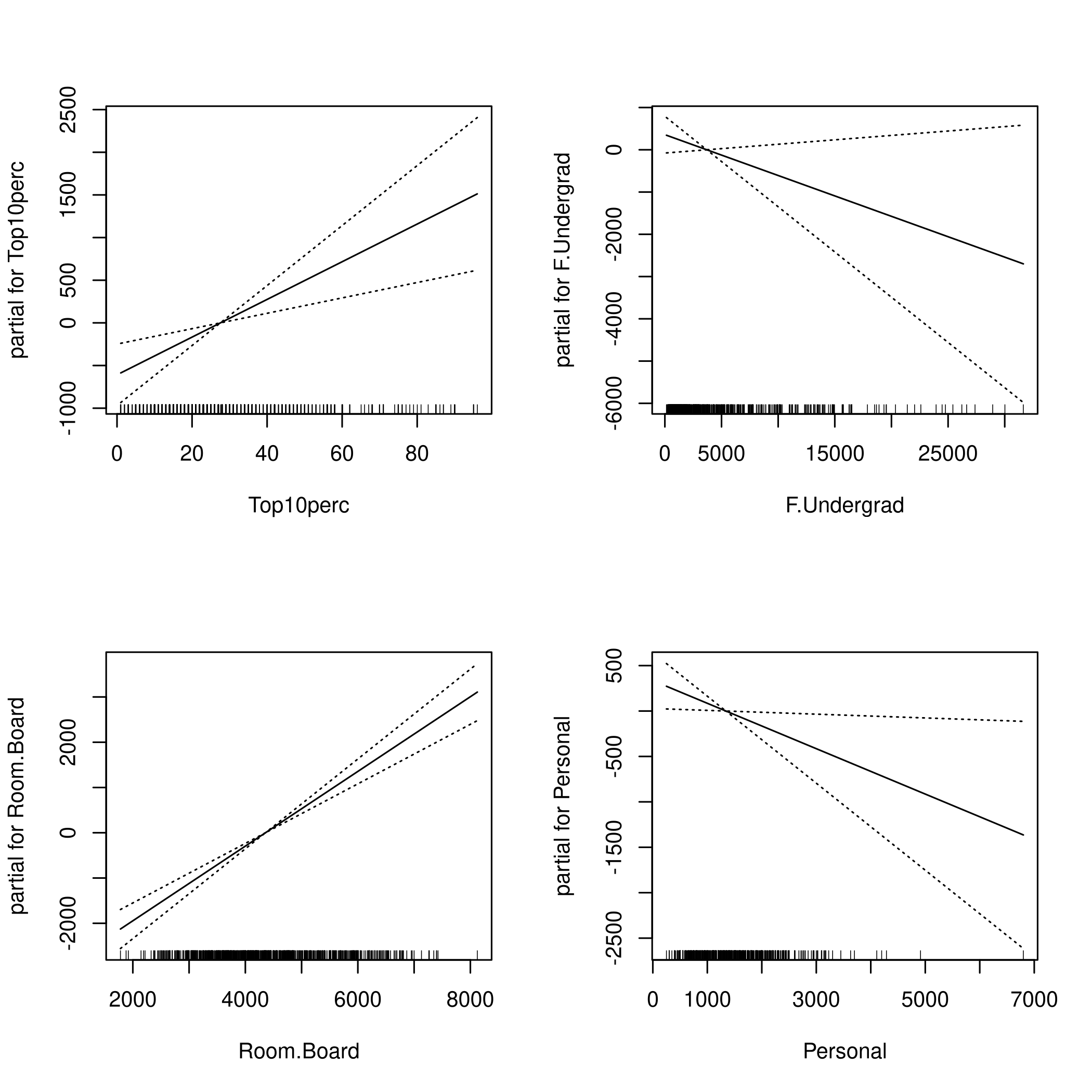
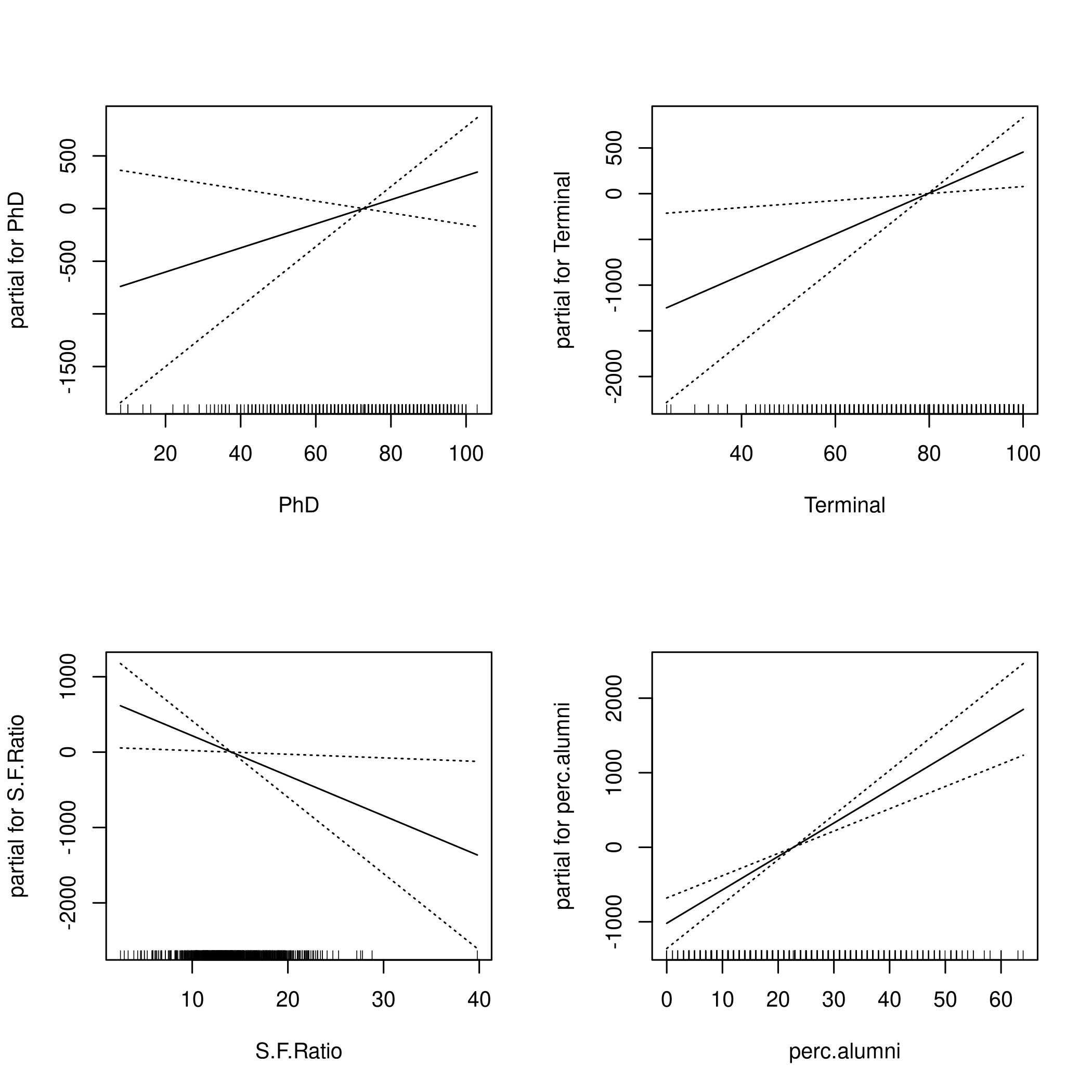
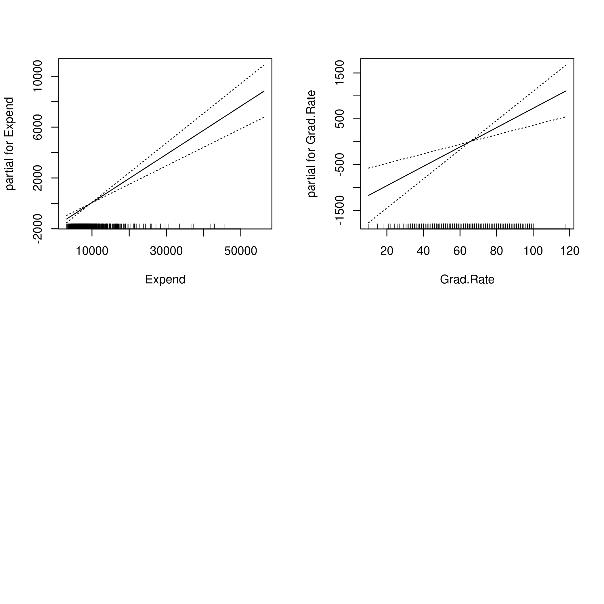
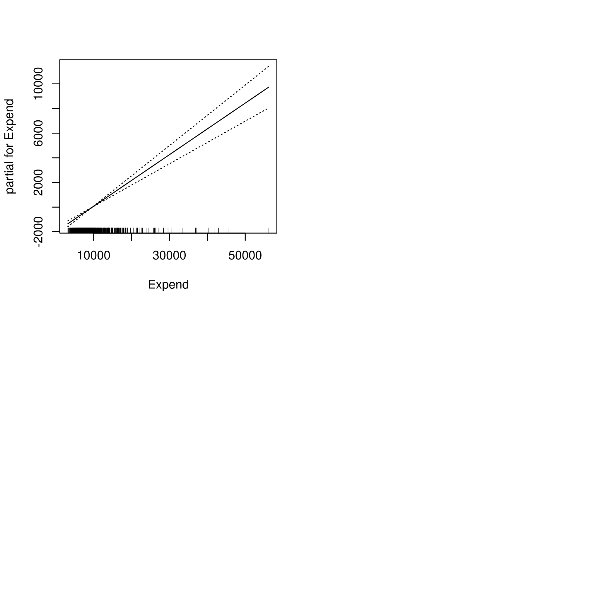
b) GAM
1library(gam)
1fit = gam(Outstate ~ Private+s(Apps,3)+Accept+Enroll+
2            Top10perc+F.Undergrad+Room.Board+
3            Personal+PhD+Terminal+S.F.Ratio+
4            perc.alumni+Expend+Grad.Rate
5        , data = colDat)
1## Warning in model.matrix.default(mt, mf, contrasts): non-list contrasts argument
2## ignored
1fit2 = gam(Outstate ~ Private+s(Room.Board,2)+s(PhD,3)+s(perc.alumni)+Expend
2        , data = colDat)
1## Warning in model.matrix.default(mt, mf, contrasts): non-list contrasts argument
2## ignored
1par(mfrow=c(2,2))
2plot(fit,se=TRUE)
1par(mfrow=c(2,2))
2plot(fit2,se=TRUE)
c) Evaluate
1pred <- predict(fit, test_set)
2mse.error <- mean((test_set$Outstate - pred)^2)
3mse.error %>% print
1## [1] 3691891
1gam.tss = mean((test_set$Outstate - mean(test_set$Outstate))^2)
2test.rss = 1 - mse.error/gam.tss
3test.rss %>% print
1## [1] 0.7731239
1pred2 <- predict(fit2, test_set)
2mse.error2 <- mean((test_set$Outstate - pred2)^2)
3mse.error2 %>% print
1## [1] 4121902
1gam.tss2 = mean((test_set$Outstate - mean(test_set$Outstate))^2)
2test.rss2 = 1 - mse.error2/gam.tss2
3test.rss2 %>% print
1## [1] 0.7466987
This is pretty good model, all told.
d) Summary
1summary(fit) %>% print
 1##
 2## Call: gam(formula = Outstate ~ Private + s(Apps, 3) + Accept + Enroll +
 3##     Top10perc + F.Undergrad + Room.Board + Personal + PhD + Terminal +
 4##     S.F.Ratio + perc.alumni + Expend + Grad.Rate, data = colDat)
 5## Deviance Residuals:
 6##       Min        1Q    Median        3Q       Max
 7## -6641.083 -1262.806    -5.698  1270.911  9965.901
 8##
 9## (Dispersion Parameter for gaussian family taken to be 3749048)
10##
11##     Null Deviance: 12559297426 on 776 degrees of freedom
12## Residual Deviance: 2849276343 on 760 degrees of freedom
13## AIC: 13985.3
14##
15## Number of Local Scoring Iterations: 2
16##
17## Anova for Parametric Effects
18##              Df     Sum Sq    Mean Sq  F value    Pr(>F)
19## Private       1 4034912907 4034912907 1076.250 < 2.2e-16 ***
20## s(Apps, 3)    1 1344548030 1344548030  358.637 < 2.2e-16 ***
21## Accept        1   90544274   90544274   24.151 1.091e-06 ***
22## Enroll        1  144471570  144471570   38.535 8.838e-10 ***
23## Top10perc     1 1802244831 1802244831  480.721 < 2.2e-16 ***
24## F.Undergrad   1   45230645   45230645   12.065 0.0005430 ***
25## Room.Board    1 1110285773 1110285773  296.151 < 2.2e-16 ***
26## Personal      1   47886988   47886988   12.773 0.0003738 ***
27## PhD           1  220249039  220249039   58.748 5.476e-14 ***
28## Terminal      1   66366007   66366007   17.702 2.892e-05 ***
29## S.F.Ratio     1  190811028  190811028   50.896 2.274e-12 ***
30## perc.alumni   1  225293653  225293653   60.094 2.904e-14 ***
31## Expend        1  258162295  258162295   68.861 4.805e-16 ***
32## Grad.Rate     1   57947219   57947219   15.457 9.214e-05 ***
33## Residuals   760 2849276343    3749048
34## ---
35## Signif. codes:  0 '***' 0.001 '**' 0.01 '*' 0.05 '.' 0.1 ' ' 1
36##
37## Anova for Nonparametric Effects
38##             Npar Df Npar F     Pr(F)
39## (Intercept)
40## Private
41## s(Apps, 3)        2  8.571 0.0002085 ***
42## Accept
43## Enroll
44## Top10perc
45## F.Undergrad
46## Room.Board
47## Personal
48## PhD
49## Terminal
50## S.F.Ratio
51## perc.alumni
52## Expend
53## Grad.Rate
54## ---
55## Signif. codes:  0 '***' 0.001 '**' 0.01 '*' 0.05 '.' 0.1 ' ' 1
1summary(fit2) %>% print
 1##
 2## Call: gam(formula = Outstate ~ Private + s(Room.Board, 2) + s(PhD,
 3##     3) + s(perc.alumni) + Expend, data = colDat)
 4## Deviance Residuals:
 5##       Min        1Q    Median        3Q       Max
 6## -8676.030 -1345.678    -8.409  1265.524  9590.459
 7##
 8## (Dispersion Parameter for gaussian family taken to be 4175193)
 9##
10##     Null Deviance: 12559297426 on 776 degrees of freedom
11## Residual Deviance: 3194023899 on 765.0002 degrees of freedom
12## AIC: 14064.05
13##
14## Number of Local Scoring Iterations: 2
15##
16## Anova for Parametric Effects
17##                   Df     Sum Sq    Mean Sq F value    Pr(>F)
18## Private            1 3751107814 3751107814  898.43 < 2.2e-16 ***
19## s(Room.Board, 2)   1 2913770756 2913770756  697.88 < 2.2e-16 ***
20## s(PhD, 3)          1 1149711330 1149711330  275.37 < 2.2e-16 ***
21## s(perc.alumni)     1  556759894  556759894  133.35 < 2.2e-16 ***
22## Expend             1  554812125  554812125  132.88 < 2.2e-16 ***
23## Residuals        765 3194023899    4175193
24## ---
25## Signif. codes:  0 '***' 0.001 '**' 0.01 '*' 0.05 '.' 0.1 ' ' 1
26##
27## Anova for Nonparametric Effects
28##                  Npar Df Npar F     Pr(F)
29## (Intercept)
30## Private
31## s(Room.Board, 2)       1 4.9853 0.0258517 *
32## s(PhD, 3)              2 9.1614 0.0001171 ***
33## s(perc.alumni)         3 0.8726 0.4548496
34## Expend
35## ---
36## Signif. codes:  0 '***' 0.001 '**' 0.01 '*' 0.05 '.' 0.1 ' ' 1
James, G., Witten, D., Hastie, T., & Tibshirani, R. (2013). An Introduction to Statistical Learning: with Applications in R. Berlin, Germany: Springer Science & Business Media. ↩︎
![]()