
17 minutes
Written: 2020-06-28 00:00 +0000
SR2 :: Solutions for Chapters {13,14}
Setup details are described here, and the meta-post about these solutions is here.
Materials
The summmer course1 is based off of the second edition of Statistical Rethinking by Richard McElreath.
- Chapter 13
- E{1,2,3,4,5}
- Chapter 14
- E{1,2,3}
Packages
A colophon with details is provided at the end, but the following packages and theme parameters are used throughout.
1libsUsed<-c("tidyverse","tidybayes","orgutils","dagitty",
2            "rethinking","tidybayes.rethinking",
3            "ggplot2","kableExtra","dplyr","glue",
4            "latex2exp","data.table","printr","devtools")
5invisible(lapply(libsUsed, library, character.only = TRUE));
6theme_set(theme_grey(base_size=24))
7set.seed(1995)
Chapter XIII: Models With Memory
Easy Questions (Ch13)
HOLD 13E1
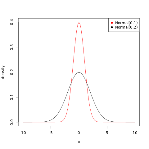
Which of the following priors will produce more shrinkage in the estimates? (a) \(α_{\mathrm{TANK}}∼\mathrm{Normal}(0,1)\); (b) \(α_{\mathrm{TANK}}∼\mathrm{Normal}(0,2)\).
Solution
The normal distribution fits a probability distribution centered around the mean and the spread is given by the standard deviation. Thus the first option, (a) will produce more shrinkage in the estimates, as the prior will be more concentrated.
1curve(dnorm(x,0,1),from=-10,to=10,col="red",ylab="density")
2curve(dnorm(x,0,2),add=TRUE)
3legend("topright",
4       col = c("red","black"),
5       pch = 19,
6       legend = c("Normal(0,1)","Normal(0,2)"))
13E2
Rewrite the following model as a multilevel model.
Solution
The model can be expressed as:
The priors have been chosen to be essentially uninformative, as is appropriate for a situation where no further insight is present for the hyperparameters.
13E3
Rewrite the following model as a multilevel model.
Solution
The model can be defined as:
HOLD 13E4
Write a mathematical model formula for a Poisson regression with varying intercepts.
Solution
13E5
Write a mathematical model formula for a Poisson regression with two different kinds of varying intercepts, a cross-classified model.
Solution
We will use the non-centered form for the cross-classified model.
Chapter XIV: Adventures in Covariance
Easy Questions (Ch14)
HOLD 14E1
Add to the following model varying slopes on the predictor \(x\).
Solution
Following the convention in the physical sciences, I will use square brackets for matrices and parenthesis for vectors.
Where we do not have any information so have used a standard weakly informative LKJcorr prior for correlation matrices which is flat for all valid correlation matrices. We also use weakly uninformative priors for the standard deviations among slopes and intercepts.
HOLD 14E2
Think up a context in which varying intercepts will be positively correlated with varying slopes. Provide a mechanistic explanation for the correlation.
Solution
We note at the onset that the concept of varying intercepts is to account for blocks or sub-groups in our problem. This means that the clusters in our data which have higher average values will show a stronger positive association with predictor variables. To augment the example of the tadpoles in the book, if the data is arranged as:
- Tadpoles in tanks
- Some tanks have larger tadpoles (different species) which grow faster
For a repeated measurement in an interval of time, there will be a positive correlation between the initial height and the slope.
HOLD 14E3
When is it possible for a varying slopes model to have fewer effective parameters (as estimated by WAIC or PSIS) than the corresponding model with fixed (unpooled) slopes? Explain.
Solution
The varying effects essentially causes regularization or shrinkage towards the global mean to prevent overfitting to the individual data-points. Consider the example from the text, for the chimpanzee experiment.
1data(chimpanzees)
2d <- chimpanzees
3d$block_id <- d$block
4d$treatment <- 1L + d$prosoc_left + 2L*d$condition
5dat <- list(
6L = d$pulled_left,
7tid = as.integer(d$treatment),
8actor = d$actor )
We will set up a simple fixed effects model.
1m14fix <- ulam(
2alist(
3L ~ dbinom( 1 , p ) ,
4logit(p) <- alpha[actor] + beta[tid] ,
5alpha[actor] ~ dnorm( 0 , 5 ),
6beta[tid] ~ dnorm( 0 , 0.5 )
7) , data=dat , chains=4 , log_lik=TRUE )
 1SAMPLING FOR MODEL '90fe1cae14bc2bf32f08b4d71c2d1f0d' NOW (CHAIN 1).
 2Chain 1:
 3Chain 1: Gradient evaluation took 9.2e-05 seconds
 4Chain 1: 1000 transitions using 10 leapfrog steps per transition would take 0.92 seconds.
 5Chain 1: Adjust your expectations accordingly!
 6Chain 1:
 7Chain 1:
 8Chain 1: Iteration:   1 / 1000 [  0%]  (Warmup)
 9Chain 1: Iteration: 100 / 1000 [ 10%]  (Warmup)
10Chain 1: Iteration: 200 / 1000 [ 20%]  (Warmup)
11Chain 1: Iteration: 300 / 1000 [ 30%]  (Warmup)
12Chain 1: Iteration: 400 / 1000 [ 40%]  (Warmup)
13Chain 1: Iteration: 500 / 1000 [ 50%]  (Warmup)
14Chain 1: Iteration: 501 / 1000 [ 50%]  (Sampling)
15Chain 1: Iteration: 600 / 1000 [ 60%]  (Sampling)
16Chain 1: Iteration: 700 / 1000 [ 70%]  (Sampling)
17Chain 1: Iteration: 800 / 1000 [ 80%]  (Sampling)
18Chain 1: Iteration: 900 / 1000 [ 90%]  (Sampling)
19Chain 1: Iteration: 1000 / 1000 [100%]  (Sampling)
20Chain 1:
21Chain 1:  Elapsed Time: 0.335488 seconds (Warm-up)
22Chain 1:                0.228533 seconds (Sampling)
23Chain 1:                0.564021 seconds (Total)
24Chain 1:
25
26SAMPLING FOR MODEL '90fe1cae14bc2bf32f08b4d71c2d1f0d' NOW (CHAIN 2).
27Chain 2:
28Chain 2: Gradient evaluation took 3.4e-05 seconds
29Chain 2: 1000 transitions using 10 leapfrog steps per transition would take 0.34 seconds.
30Chain 2: Adjust your expectations accordingly!
31Chain 2:
32Chain 2:
33Chain 2: Iteration:   1 / 1000 [  0%]  (Warmup)
34Chain 2: Iteration: 100 / 1000 [ 10%]  (Warmup)
35Chain 2: Iteration: 200 / 1000 [ 20%]  (Warmup)
36Chain 2: Iteration: 300 / 1000 [ 30%]  (Warmup)
37Chain 2: Iteration: 400 / 1000 [ 40%]  (Warmup)
38Chain 2: Iteration: 500 / 1000 [ 50%]  (Warmup)
39Chain 2: Iteration: 501 / 1000 [ 50%]  (Sampling)
40Chain 2: Iteration: 600 / 1000 [ 60%]  (Sampling)
41Chain 2: Iteration: 700 / 1000 [ 70%]  (Sampling)
42Chain 2: Iteration: 800 / 1000 [ 80%]  (Sampling)
43Chain 2: Iteration: 900 / 1000 [ 90%]  (Sampling)
44Chain 2: Iteration: 1000 / 1000 [100%]  (Sampling)
45Chain 2:
46Chain 2:  Elapsed Time: 0.365676 seconds (Warm-up)
47Chain 2:                0.330942 seconds (Sampling)
48Chain 2:                0.696618 seconds (Total)
49Chain 2:
50
51SAMPLING FOR MODEL '90fe1cae14bc2bf32f08b4d71c2d1f0d' NOW (CHAIN 3).
52Chain 3:
53Chain 3: Gradient evaluation took 4.3e-05 seconds
54Chain 3: 1000 transitions using 10 leapfrog steps per transition would take 0.43 seconds.
55Chain 3: Adjust your expectations accordingly!
56Chain 3:
57Chain 3:
58Chain 3: Iteration:   1 / 1000 [  0%]  (Warmup)
59Chain 3: Iteration: 100 / 1000 [ 10%]  (Warmup)
60Chain 3: Iteration: 200 / 1000 [ 20%]  (Warmup)
61Chain 3: Iteration: 300 / 1000 [ 30%]  (Warmup)
62Chain 3: Iteration: 400 / 1000 [ 40%]  (Warmup)
63Chain 3: Iteration: 500 / 1000 [ 50%]  (Warmup)
64Chain 3: Iteration: 501 / 1000 [ 50%]  (Sampling)
65Chain 3: Iteration: 600 / 1000 [ 60%]  (Sampling)
66Chain 3: Iteration: 700 / 1000 [ 70%]  (Sampling)
67Chain 3: Iteration: 800 / 1000 [ 80%]  (Sampling)
68Chain 3: Iteration: 900 / 1000 [ 90%]  (Sampling)
69Chain 3: Iteration: 1000 / 1000 [100%]  (Sampling)
70Chain 3:
71Chain 3:  Elapsed Time: 0.356879 seconds (Warm-up)
72Chain 3:                0.352045 seconds (Sampling)
73Chain 3:                0.708924 seconds (Total)
74Chain 3:
75
76SAMPLING FOR MODEL '90fe1cae14bc2bf32f08b4d71c2d1f0d' NOW (CHAIN 4).
77Chain 4:
78Chain 4: Gradient evaluation took 4.5e-05 seconds
79Chain 4: 1000 transitions using 10 leapfrog steps per transition would take 0.45 seconds.
80Chain 4: Adjust your expectations accordingly!
81Chain 4:
82Chain 4:
83Chain 4: Iteration:   1 / 1000 [  0%]  (Warmup)
84Chain 4: Iteration: 100 / 1000 [ 10%]  (Warmup)
85Chain 4: Iteration: 200 / 1000 [ 20%]  (Warmup)
86Chain 4: Iteration: 300 / 1000 [ 30%]  (Warmup)
87Chain 4: Iteration: 400 / 1000 [ 40%]  (Warmup)
88Chain 4: Iteration: 500 / 1000 [ 50%]  (Warmup)
89Chain 4: Iteration: 501 / 1000 [ 50%]  (Sampling)
90Chain 4: Iteration: 600 / 1000 [ 60%]  (Sampling)
91Chain 4: Iteration: 700 / 1000 [ 70%]  (Sampling)
92Chain 4: Iteration: 800 / 1000 [ 80%]  (Sampling)
93Chain 4: Iteration: 900 / 1000 [ 90%]  (Sampling)
94Chain 4: Iteration: 1000 / 1000 [100%]  (Sampling)
95Chain 4:
96Chain 4:  Elapsed Time: 0.296276 seconds (Warm-up)
97Chain 4:                0.261692 seconds (Sampling)
98Chain 4:                0.557968 seconds (Total)
99Chain 4:
Now we can extend this to a varying slopes model, where we will consider varying slopes for actors.
1m14ppool <- ulam(
2alist(
3L ~ dbinom( 1 , p ) ,
4logit(p) <- alpha + a[actor]*vary_id + beta[tid],
5alpha ~ dnorm( 0 , 5 ),
6a[actor] ~ dnorm( 0 , 1 ),
7beta[tid] ~ dnorm( 0 , 0.5 ),
8vary_id ~ dexp( 1 )
9) , data=dat , chains=4 , log_lik=TRUE )
 1SAMPLING FOR MODEL 'd14d0bbe9399ac4de917b8e279a6e9e5' NOW (CHAIN 1).
 2Chain 1:
 3Chain 1: Gradient evaluation took 0.000184 seconds
 4Chain 1: 1000 transitions using 10 leapfrog steps per transition would take 1.84 seconds.
 5Chain 1: Adjust your expectations accordingly!
 6Chain 1:
 7Chain 1:
 8Chain 1: Iteration:   1 / 1000 [  0%]  (Warmup)
 9Chain 1: Iteration: 100 / 1000 [ 10%]  (Warmup)
10Chain 1: Iteration: 200 / 1000 [ 20%]  (Warmup)
11Chain 1: Iteration: 300 / 1000 [ 30%]  (Warmup)
12Chain 1: Iteration: 400 / 1000 [ 40%]  (Warmup)
13Chain 1: Iteration: 500 / 1000 [ 50%]  (Warmup)
14Chain 1: Iteration: 501 / 1000 [ 50%]  (Sampling)
15Chain 1: Iteration: 600 / 1000 [ 60%]  (Sampling)
16Chain 1: Iteration: 700 / 1000 [ 70%]  (Sampling)
17Chain 1: Iteration: 800 / 1000 [ 80%]  (Sampling)
18Chain 1: Iteration: 900 / 1000 [ 90%]  (Sampling)
19Chain 1: Iteration: 1000 / 1000 [100%]  (Sampling)
20Chain 1:
21Chain 1:  Elapsed Time: 1.63295 seconds (Warm-up)
22Chain 1:                1.18708 seconds (Sampling)
23Chain 1:                2.82003 seconds (Total)
24Chain 1:
25
26SAMPLING FOR MODEL 'd14d0bbe9399ac4de917b8e279a6e9e5' NOW (CHAIN 2).
27Chain 2:
28Chain 2: Gradient evaluation took 6.3e-05 seconds
29Chain 2: 1000 transitions using 10 leapfrog steps per transition would take 0.63 seconds.
30Chain 2: Adjust your expectations accordingly!
31Chain 2:
32Chain 2:
33Chain 2: Iteration:   1 / 1000 [  0%]  (Warmup)
34Chain 2: Iteration: 100 / 1000 [ 10%]  (Warmup)
35Chain 2: Iteration: 200 / 1000 [ 20%]  (Warmup)
36Chain 2: Iteration: 300 / 1000 [ 30%]  (Warmup)
37Chain 2: Iteration: 400 / 1000 [ 40%]  (Warmup)
38Chain 2: Iteration: 500 / 1000 [ 50%]  (Warmup)
39Chain 2: Iteration: 501 / 1000 [ 50%]  (Sampling)
40Chain 2: Iteration: 600 / 1000 [ 60%]  (Sampling)
41Chain 2: Iteration: 700 / 1000 [ 70%]  (Sampling)
42Chain 2: Iteration: 800 / 1000 [ 80%]  (Sampling)
43Chain 2: Iteration: 900 / 1000 [ 90%]  (Sampling)
44Chain 2: Iteration: 1000 / 1000 [100%]  (Sampling)
45Chain 2:
46Chain 2:  Elapsed Time: 1.58303 seconds (Warm-up)
47Chain 2:                1.30156 seconds (Sampling)
48Chain 2:                2.88459 seconds (Total)
49Chain 2:
50
51SAMPLING FOR MODEL 'd14d0bbe9399ac4de917b8e279a6e9e5' NOW (CHAIN 3).
52Chain 3:
53Chain 3: Gradient evaluation took 6.4e-05 seconds
54Chain 3: 1000 transitions using 10 leapfrog steps per transition would take 0.64 seconds.
55Chain 3: Adjust your expectations accordingly!
56Chain 3:
57Chain 3:
58Chain 3: Iteration:   1 / 1000 [  0%]  (Warmup)
59Chain 3: Iteration: 100 / 1000 [ 10%]  (Warmup)
60Chain 3: Iteration: 200 / 1000 [ 20%]  (Warmup)
61Chain 3: Iteration: 300 / 1000 [ 30%]  (Warmup)
62Chain 3: Iteration: 400 / 1000 [ 40%]  (Warmup)
63Chain 3: Iteration: 500 / 1000 [ 50%]  (Warmup)
64Chain 3: Iteration: 501 / 1000 [ 50%]  (Sampling)
65Chain 3: Iteration: 600 / 1000 [ 60%]  (Sampling)
66Chain 3: Iteration: 700 / 1000 [ 70%]  (Sampling)
67Chain 3: Iteration: 800 / 1000 [ 80%]  (Sampling)
68Chain 3: Iteration: 900 / 1000 [ 90%]  (Sampling)
69Chain 3: Iteration: 1000 / 1000 [100%]  (Sampling)
70Chain 3:
71Chain 3:  Elapsed Time: 1.37077 seconds (Warm-up)
72Chain 3:                1.12109 seconds (Sampling)
73Chain 3:                2.49186 seconds (Total)
74Chain 3:
75
76SAMPLING FOR MODEL 'd14d0bbe9399ac4de917b8e279a6e9e5' NOW (CHAIN 4).
77Chain 4:
78Chain 4: Gradient evaluation took 5.9e-05 seconds
79Chain 4: 1000 transitions using 10 leapfrog steps per transition would take 0.59 seconds.
80Chain 4: Adjust your expectations accordingly!
81Chain 4:
82Chain 4:
83Chain 4: Iteration:   1 / 1000 [  0%]  (Warmup)
84Chain 4: Iteration: 100 / 1000 [ 10%]  (Warmup)
85Chain 4: Iteration: 200 / 1000 [ 20%]  (Warmup)
86Chain 4: Iteration: 300 / 1000 [ 30%]  (Warmup)
87Chain 4: Iteration: 400 / 1000 [ 40%]  (Warmup)
88Chain 4: Iteration: 500 / 1000 [ 50%]  (Warmup)
89Chain 4: Iteration: 501 / 1000 [ 50%]  (Sampling)
90Chain 4: Iteration: 600 / 1000 [ 60%]  (Sampling)
91Chain 4: Iteration: 700 / 1000 [ 70%]  (Sampling)
92Chain 4: Iteration: 800 / 1000 [ 80%]  (Sampling)
93Chain 4: Iteration: 900 / 1000 [ 90%]  (Sampling)
94Chain 4: Iteration: 1000 / 1000 [100%]  (Sampling)
95Chain 4:
96Chain 4:  Elapsed Time: 1.48561 seconds (Warm-up)
97Chain 4:                1.38809 seconds (Sampling)
98Chain 4:                2.8737 seconds (Total)
99Chain 4:
Now we can test the number of parameters.
1compare(m14ppool,m14fix) %>% toOrg
1| row.names |             WAIC |               SE |            dWAIC |              dSE |            pWAIC |            weight |
2|-----------+------------------+------------------+------------------+------------------+------------------+-------------------|
3| m14ppool  | 532.211705503729 | 19.5177343184252 |                0 |               NA | 9.12911563615787 | 0.796616007296431 |
4| m14fix    | 534.942259470042 | 18.0912938913487 | 2.73055396631241 | 1.66292448384092 | 8.10370201332515 | 0.203383992703568 |
As we can see, the model with partial pooling has only one effective additional parameter, even though the model without pooling has \(n(\mathrm{actor})\) intercepts (one per actor) with a standard deviation, while the partial pooling parameter has an additional average intercept and a standard deviation parameter.
Both the models have around the same number of effective parameters, which mean that the additional parameters do not actually cause additional overfitting. This simply implies that for Bayesian models, the raw number of model parameters does not correspond necessarily to a model with more overfitting.
In general, we should keep in mind that the effective number of parameters, when the variation among clusters is high, is probably going to be lower than the total number of parameters, due to adaptive regularization.
A: Colophon
To ensure that this document is fully reproducible at a later date, we will record the session info.
1devtools::session_info()
  1─ Session info ───────────────────────────────────────────────────────────────
  2 setting  value
  3 version  R version 4.0.0 (2020-04-24)
  4 os       Arch Linux
  5 system   x86_64, linux-gnu
  6 ui       X11
  7 language (EN)
  8 collate  en_US.UTF-8
  9 ctype    en_US.UTF-8
 10 tz       Iceland
 11 date     2020-06-27
 12
 13─ Packages ───────────────────────────────────────────────────────────────────
 14 package              * version    date       lib   source
 15 arrayhelpers           1.1-0      2020-02-04 [167] CRAN (R 4.0.0)
 16 assertthat             0.2.1      2019-03-21 [34]  CRAN (R 4.0.0)
 17 backports              1.1.6      2020-04-05 [68]  CRAN (R 4.0.0)
 18 boot                   1.3-24     2019-12-20 [5]   CRAN (R 4.0.0)
 19 broom                  0.5.6      2020-04-20 [67]  CRAN (R 4.0.0)
 20 callr                  3.4.3      2020-03-28 [87]  CRAN (R 4.0.0)
 21 cellranger             1.1.0      2016-07-27 [55]  CRAN (R 4.0.0)
 22 cli                    2.0.2      2020-02-28 [33]  CRAN (R 4.0.0)
 23 coda                   0.19-3     2019-07-05 [169] CRAN (R 4.0.0)
 24 colorspace             1.4-1      2019-03-18 [97]  CRAN (R 4.0.0)
 25 crayon                 1.3.4      2017-09-16 [35]  CRAN (R 4.0.0)
 26 curl                   4.3        2019-12-02 [26]  CRAN (R 4.0.0)
 27 dagitty              * 0.2-2      2016-08-26 [244] CRAN (R 4.0.0)
 28 data.table           * 1.12.8     2019-12-09 [27]  CRAN (R 4.0.0)
 29 DBI                    1.1.0      2019-12-15 [77]  CRAN (R 4.0.0)
 30 dbplyr                 1.4.3      2020-04-19 [76]  CRAN (R 4.0.0)
 31 desc                   1.2.0      2018-05-01 [84]  CRAN (R 4.0.0)
 32 devtools             * 2.3.0      2020-04-10 [219] CRAN (R 4.0.0)
 33 digest                 0.6.25     2020-02-23 [42]  CRAN (R 4.0.0)
 34 dplyr                * 0.8.5      2020-03-07 [69]  CRAN (R 4.0.0)
 35 ellipsis               0.3.0      2019-09-20 [30]  CRAN (R 4.0.0)
 36 evaluate               0.14       2019-05-28 [82]  CRAN (R 4.0.0)
 37 fansi                  0.4.1      2020-01-08 [36]  CRAN (R 4.0.0)
 38 forcats              * 0.5.0      2020-03-01 [29]  CRAN (R 4.0.0)
 39 fs                     1.4.1      2020-04-04 [109] CRAN (R 4.0.0)
 40 generics               0.0.2      2018-11-29 [71]  CRAN (R 4.0.0)
 41 ggplot2              * 3.3.0      2020-03-05 [78]  CRAN (R 4.0.0)
 42 glue                 * 1.4.0      2020-04-03 [37]  CRAN (R 4.0.0)
 43 gridExtra              2.3        2017-09-09 [123] CRAN (R 4.0.0)
 44 gtable                 0.3.0      2019-03-25 [79]  CRAN (R 4.0.0)
 45 haven                  2.2.0      2019-11-08 [28]  CRAN (R 4.0.0)
 46 hms                    0.5.3      2020-01-08 [44]  CRAN (R 4.0.0)
 47 htmltools              0.4.0      2019-10-04 [112] CRAN (R 4.0.0)
 48 httr                   1.4.1      2019-08-05 [100] CRAN (R 4.0.0)
 49 inline                 0.3.15     2018-05-18 [162] CRAN (R 4.0.0)
 50 jsonlite               1.6.1      2020-02-02 [101] CRAN (R 4.0.0)
 51 kableExtra           * 1.1.0      2019-03-16 [212] CRAN (R 4.0.0)
 52 knitr                  1.28       2020-02-06 [113] CRAN (R 4.0.0)
 53 latex2exp            * 0.4.0      2015-11-30 [211] CRAN (R 4.0.0)
 54 lattice                0.20-41    2020-04-02 [6]   CRAN (R 4.0.0)
 55 lifecycle              0.2.0      2020-03-06 [38]  CRAN (R 4.0.0)
 56 loo                    2.2.0      2019-12-19 [163] CRAN (R 4.0.0)
 57 lubridate              1.7.8      2020-04-06 [106] CRAN (R 4.0.0)
 58 magrittr               1.5        2014-11-22 [21]  CRAN (R 4.0.0)
 59 MASS                   7.3-51.5   2019-12-20 [7]   CRAN (R 4.0.0)
 60 matrixStats            0.56.0     2020-03-13 [164] CRAN (R 4.0.0)
 61 memoise                1.1.0      2017-04-21 [229] CRAN (R 4.0.0)
 62 modelr                 0.1.6      2020-02-22 [107] CRAN (R 4.0.0)
 63 munsell                0.5.0      2018-06-12 [96]  CRAN (R 4.0.0)
 64 mvtnorm                1.1-0      2020-02-24 [243] CRAN (R 4.0.0)
 65 nlme                   3.1-147    2020-04-13 [11]  CRAN (R 4.0.0)
 66 orgutils             * 0.4-1      2017-03-21 [209] CRAN (R 4.0.0)
 67 pillar                 1.4.3      2019-12-20 [39]  CRAN (R 4.0.0)
 68 pkgbuild               1.0.6      2019-10-09 [86]  CRAN (R 4.0.0)
 69 pkgconfig              2.0.3      2019-09-22 [43]  CRAN (R 4.0.0)
 70 pkgload                1.0.2      2018-10-29 [83]  CRAN (R 4.0.0)
 71 plyr                   1.8.6      2020-03-03 [73]  CRAN (R 4.0.0)
 72 prettyunits            1.1.1      2020-01-24 [58]  CRAN (R 4.0.0)
 73 printr               * 0.1        2017-05-19 [214] CRAN (R 4.0.0)
 74 processx               3.4.2      2020-02-09 [88]  CRAN (R 4.0.0)
 75 ps                     1.3.2      2020-02-13 [89]  CRAN (R 4.0.0)
 76 purrr                * 0.3.4      2020-04-17 [50]  CRAN (R 4.0.0)
 77 R6                     2.4.1      2019-11-12 [48]  CRAN (R 4.0.0)
 78 Rcpp                   1.0.4.6    2020-04-09 [10]  CRAN (R 4.0.0)
 79 readr                * 1.3.1      2018-12-21 [45]  CRAN (R 4.0.0)
 80 readxl                 1.3.1      2019-03-13 [54]  CRAN (R 4.0.0)
 81 remotes                2.1.1      2020-02-15 [233] CRAN (R 4.0.0)
 82 reprex                 0.3.0      2019-05-16 [108] CRAN (R 4.0.0)
 83 rethinking           * 2.01       2020-06-06 [242] local
 84 rlang                  0.4.5      2020-03-01 [31]  CRAN (R 4.0.0)
 85 rmarkdown              2.1        2020-01-20 [110] CRAN (R 4.0.0)
 86 rprojroot              1.3-2      2018-01-03 [85]  CRAN (R 4.0.0)
 87 rstan                * 2.19.3     2020-02-11 [161] CRAN (R 4.0.0)
 88 rstudioapi             0.11       2020-02-07 [91]  CRAN (R 4.0.0)
 89 rvest                  0.3.5      2019-11-08 [120] CRAN (R 4.0.0)
 90 scales                 1.1.0      2019-11-18 [93]  CRAN (R 4.0.0)
 91 sessioninfo            1.1.1      2018-11-05 [231] CRAN (R 4.0.0)
 92 shape                  1.4.4      2018-02-07 [193] CRAN (R 4.0.0)
 93 StanHeaders          * 2.19.2     2020-02-11 [165] CRAN (R 4.0.0)
 94 stringi                1.4.6      2020-02-17 [52]  CRAN (R 4.0.0)
 95 stringr              * 1.4.0      2019-02-10 [74]  CRAN (R 4.0.0)
 96 svUnit                 1.0.3      2020-04-20 [168] CRAN (R 4.0.0)
 97 testthat               2.3.2      2020-03-02 [81]  CRAN (R 4.0.0)
 98 textutils              0.2-0      2020-01-07 [210] CRAN (R 4.0.0)
 99 tibble               * 3.0.1      2020-04-20 [32]  CRAN (R 4.0.0)
100 tidybayes            * 2.0.3      2020-04-04 [166] CRAN (R 4.0.0)
101 tidybayes.rethinking * 2.0.3.9000 2020-06-07 [246] local
102 tidyr                * 1.0.2      2020-01-24 [75]  CRAN (R 4.0.0)
103 tidyselect             1.0.0      2020-01-27 [49]  CRAN (R 4.0.0)
104 tidyverse            * 1.3.0      2019-11-21 [66]  CRAN (R 4.0.0)
105 usethis              * 1.6.0      2020-04-09 [238] CRAN (R 4.0.0)
106 V8                     3.0.2      2020-03-14 [245] CRAN (R 4.0.0)
107 vctrs                  0.2.4      2020-03-10 [41]  CRAN (R 4.0.0)
108 viridisLite            0.3.0      2018-02-01 [99]  CRAN (R 4.0.0)
109 webshot                0.5.2      2019-11-22 [213] CRAN (R 4.0.0)
110 withr                  2.2.0      2020-04-20 [90]  CRAN (R 4.0.0)
111 xfun                   0.13       2020-04-13 [116] CRAN (R 4.0.0)
112 xml2                   1.3.2      2020-04-23 [122] CRAN (R 4.0.0)
113
114[1] /nix/store/xzd8h53xkyvfm3kvj5ab6znp685wi04w-r-car-3.0-7/library
115[2] /nix/store/mhr8zw9bmxarc3n821b83i0gz2j9zlrq-r-abind-1.4-5/library
116[3] /nix/store/hp86nhr0787vib3l8mkw0gf9nxwb45im-r-carData-3.0-3/library
117[4] /nix/store/vhw7s2h5ds6sp110z2yvilchv8j9jch5-r-lme4-1.1-23/library
118[5] /nix/store/987n8g0zy9sjvfvnsck1bkkcknw05yvb-r-boot-1.3-24/library
119[6] /nix/store/jxxxxyz4c1k5g3drd35gsrbjdg028d11-r-lattice-0.20-41/library
120[7] /nix/store/q9zfm5h53m8rd08xcsdcwaag31k4z1pf-r-MASS-7.3-51.5/library
121[8] /nix/store/kjkm50sr144yvrhl5axfgykbiy13pbmg-r-Matrix-1.2-18/library
122[9] /nix/store/8786z5lgy8h3akfjgj3yq5yq4s17rhjy-r-minqa-1.2.4/library
123[10] /nix/store/93wv3j0z1nzqp6fjsm9v7v8bf8d1xkm2-r-Rcpp-1.0.4.6/library
124[11] /nix/store/akfw6zsmawmz8lmjkww0rnqrazm4mqp0-r-nlme-3.1-147/library
125[12] /nix/store/rxs0d9bbn8qhw7wmkfb21yk5abp6lpq1-r-nloptr-1.2.2.1/library
126[13] /nix/store/8n0jfiqn4275i58qgld0dv8zdaihdzrk-r-RcppEigen-0.3.3.7.0/library
127[14] /nix/store/8vxrma33rhc96260zsi1jiw7dy3v2mm4-r-statmod-1.4.34/library
128[15] /nix/store/2y46pb5x9lh8m0hdmzajnx7sc1bk9ihl-r-maptools-0.9-9/library
129[16] /nix/store/iwf9nxx1v883wlv0p88q947hpz5lhfh7-r-foreign-0.8-78/library
130[17] /nix/store/rl9sjqply6rjbnz5k792ghm62ybv76px-r-sp-1.4-1/library
131[18] /nix/store/ws4bkzyv2vj5pyn1hgwyy6nlp48arz0n-r-mgcv-1.8-31/library
132[19] /nix/store/307dzxrmnqk4p86560a02r64x1fhhmxb-r-nnet-7.3-13/library
133[20] /nix/store/g2zpzkdb9hzkza1wpcbrk58119v1wyaf-r-pbkrtest-0.4-8.6/library
134[21] /nix/store/p0l503fr8960vld70w6ilmknxs5qwq77-r-magrittr-1.5/library
135[22] /nix/store/rmjpcaw3i446kwnjgcxcaid0yac36cj2-r-quantreg-5.55/library
136[23] /nix/store/10mzmnvc5jjgk2xzasia522pk60a30qz-r-MatrixModels-0.4-1/library
137[24] /nix/store/6qwdzvmnnmhjwdnvg2zmvv6wafd1vf91-r-SparseM-1.78/library
138[25] /nix/store/aa9c39a3yiqkh1h7pbngjlbr7czvc7yi-r-rio-0.5.16/library
139[26] /nix/store/2fx4vqlybgwp5rhhy6pssqx7h1a927fn-r-curl-4.3/library
140[27] /nix/store/k4m3fn1kqvvvn8y33kd57gq49hr3ar8y-r-data.table-1.12.8/library
141[28] /nix/store/651hfjylqzmsf565wyx474vyjny771gy-r-haven-2.2.0/library
142[29] /nix/store/a3rnz28irmqvmj8axj5x5j1am2c3gzs4-r-forcats-0.5.0/library
143[30] /nix/store/j8v4gzib137q2cml31hvvfkrc0f60pp5-r-ellipsis-0.3.0/library
144[31] /nix/store/xaswqlnamf4k8vwx0x3wav3l0x60sag0-r-rlang-0.4.5/library
145[32] /nix/store/dqm3xpix2jwhhhr67s6fgrwbw7hizap7-r-tibble-3.0.1/library
146[33] /nix/store/v7xfsq6d97wpn6m0hjrac78w5xawbr8a-r-cli-2.0.2/library
147[34] /nix/store/fikjasr98klhk9cf44x4lhi57vh3pmkg-r-assertthat-0.2.1/library
148[35] /nix/store/3fya6cd38vsqdj0gjb7bcsy00sirlyw1-r-crayon-1.3.4/library
149[36] /nix/store/payqi9bwh216rwhaq07jgc26l4fv1zsb-r-fansi-0.4.1/library
150[37] /nix/store/h6a61ghws7yrdxlg412xl1im37z5r28i-r-glue-1.4.0/library
151[38] /nix/store/y8mjbia1wbnq26dkigr0p3xxwrbzsc2r-r-lifecycle-0.2.0/library
152[39] /nix/store/kwaghh12cnifgvcbvlv2anx0hd5f4ild-r-pillar-1.4.3/library
153[40] /nix/store/k1phn8j10nni7gzvcgp0vc25dby6bb77-r-utf8-1.1.4/library
154[41] /nix/store/k3b77y8v7zsshpp1ccs8jwk2i2g4rm9a-r-vctrs-0.2.4/library
155[42] /nix/store/iibjmbh7vj0d0bfafz98yn29ymg43gkw-r-digest-0.6.25/library
156[43] /nix/store/aqsj4k3pgm80qk4jjg7sh3ac28n6alv0-r-pkgconfig-2.0.3/library
157[44] /nix/store/i7c5v8s4hd9rlqah3bbvy06yywjqwdgk-r-hms-0.5.3/library
158[45] /nix/store/2fyrk58cmcbrxid66rbwjli7y114lvrm-r-readr-1.3.1/library
159[46] /nix/store/163xq2g5nblqgh7qhvzb6mvgg6qdrirj-r-BH-1.72.0-3/library
160[47] /nix/store/dr27b6k49prwgrjs0v30b6mf5lxa36pk-r-clipr-0.7.0/library
161[48] /nix/store/bghvqg9mcaj2jkbwpy0di6c563v24acz-r-R6-2.4.1/library
162[49] /nix/store/nq8jdq7nlg9xns4xpgyj6sqv8p4ny1wz-r-tidyselect-1.0.0/library
163[50] /nix/store/zlwhf75qld7vmwx3d4bdws057ld4mqbp-r-purrr-0.3.4/library
164[51] /nix/store/0gbmmnbpqlr69l573ymkcx8154fvlaca-r-openxlsx-4.1.4/library
165[52] /nix/store/1m1q4rmwx56dvx9rdzfsfq0jpw3hw0yx-r-stringi-1.4.6/library
166[53] /nix/store/mhy5vnvbsl4q7dcinwx3vqlyywxphbfd-r-zip-2.0.4/library
167[54] /nix/store/88sp7f7q577i6l5jjanqiv5ak6nv5357-r-readxl-1.3.1/library
168[55] /nix/store/6q9zwivzalhmzdracc8ma932wirq8rl5-r-cellranger-1.1.0/library
169[56] /nix/store/jh2n6k2ancdzqych5ix8n4rq9w514qq9-r-rematch-1.0.1/library
170[57] /nix/store/22xjqikqd6q556absb5224sbx6q0kp0c-r-progress-1.2.2/library
171[58] /nix/store/9vp32wa1qvv6lkq6p70qlli5whrxzfbi-r-prettyunits-1.1.1/library
172[59] /nix/store/r9rhqb6fsk75shihmb7nagqb51pqwp0y-r-class-7.3-16/library
173[60] /nix/store/z1kad071y43wij1ml9lpghh7jbimmcli-r-cluster-2.1.0/library
174[61] /nix/store/i8wr965caf6j1rxs2dsvpzhlh4hyyb4y-r-codetools-0.2-16/library
175[62] /nix/store/8iglq3zr68a39hzswvzxqi2ffhpw9p51-r-KernSmooth-2.23-16/library
176[63] /nix/store/n3k50zv40i40drpdf8npbmy2y08gkr6w-r-rpart-4.1-15/library
177[64] /nix/store/b4r6adzcvpm8ivflsmis7ja7q4r5hkjy-r-spatial-7.3-11/library
178[65] /nix/store/zqg6hmrncl8ax3vn7z5drf4csddwnhcx-r-survival-3.1-12/library
179[66] /nix/store/4anrihkx11h8mzb269xdyi84yp5v7grl-r-tidyverse-1.3.0/library
180[67] /nix/store/945haq0w8nfm9ib7r0nfngn5lk2i15ix-r-broom-0.5.6/library
181[68] /nix/store/52viqxzrmxl7dk0zji293g5b0b9grwh8-r-backports-1.1.6/library
182[69] /nix/store/zp1k42sw2glqy51w4hnzsjs8rgi8xzx2-r-dplyr-0.8.5/library
183[70] /nix/store/mkjd98mnshch2pwnj6h31czclqdaph3f-r-plogr-0.2.0/library
184[71] /nix/store/kflrzax6y5pwfqwzgfvqz433a3q3hnhn-r-generics-0.0.2/library
185[72] /nix/store/xi1n5h5w17c33y6ax3dfhg2hgzjl9bxz-r-reshape2-1.4.4/library
186[73] /nix/store/vn63z92zkpbaxmmhzpb6mq2fvg0xa26h-r-plyr-1.8.6/library
187[74] /nix/store/wmpyxss67bj44rin7hlnr9qabx66p5hj-r-stringr-1.4.0/library
188[75] /nix/store/330qbgbvllwz3h0i2qidrlk50y0mbgph-r-tidyr-1.0.2/library
189[76] /nix/store/cx3x4pqb65l1mhss65780hbzv9jdrzl6-r-dbplyr-1.4.3/library
190[77] /nix/store/gsj49bp3hpw9jlli3894c49amddryqsq-r-DBI-1.1.0/library
191[78] /nix/store/kvymhwp4gac0343c2yi1qvdpavx4gdn2-r-ggplot2-3.3.0/library
192[79] /nix/store/knv51jvpairvibrkkq48b6f1l2pa1cv8-r-gtable-0.3.0/library
193[80] /nix/store/158dx0ddv20ikwag2860nlg9p3hbh1zc-r-isoband-0.2.1/library
194[81] /nix/store/fprs9rp1jlhxzj7fp6l79akyf8k3p7zd-r-testthat-2.3.2/library
195[82] /nix/store/0pmlnkyn0ir3k9bvxihi1r06jyl64w3i-r-evaluate-0.14/library
196[83] /nix/store/7210bjjqn5cjndxn5isnd4vip00xhkhy-r-pkgload-1.0.2/library
197[84] /nix/store/9a12ybd74b7dns40gcfs061wv7913qjy-r-desc-1.2.0/library
198[85] /nix/store/na9pb1apa787zp7vvyz1kzym0ywjwbj0-r-rprojroot-1.3-2/library
199[86] /nix/store/pa2n7bh61qxyarn5i2ynd62k6knb1np1-r-pkgbuild-1.0.6/library
200[87] /nix/store/1hxm1m7h4272zxk9bpsaq46mvnl0dbss-r-callr-3.4.3/library
201[88] /nix/store/bigvyk6ipglbiil93zkf442nv4y3xa1x-r-processx-3.4.2/library
202[89] /nix/store/370lr0wf7qlq0m72xnmasg2iahkp2n52-r-ps-1.3.2/library
203[90] /nix/store/rr72q61d8mkd42zc5fhcd2rqjghvc141-r-withr-2.2.0/library
204[91] /nix/store/9gw77p7fmz89fa8wi1d9rvril6hd4sxy-r-rstudioapi-0.11/library
205[92] /nix/store/9x4v4pbrgmykbz2801h77yz2l0nmm5nb-r-praise-1.0.0/library
206[93] /nix/store/pf8ssb0dliw5bzsncl227agc8przb7ic-r-scales-1.1.0/library
207[94] /nix/store/095z4wgjrxn63ixvyzrj1fm1rdv6ci95-r-farver-2.0.3/library
208[95] /nix/store/5aczj4s7i9prf5i32ik5ac5baqvjwdb1-r-labeling-0.3/library
209[96] /nix/store/wch26phipzz9gxd4vbr4fynh7v28349j-r-munsell-0.5.0/library
210[97] /nix/store/3w8fh756mszhsjx5fwgwydcpn8vkwady-r-colorspace-1.4-1/library
211[98] /nix/store/8cmaj81v2vm4f8p59ylbnsby8adkbmhd-r-RColorBrewer-1.1-2/library
212[99] /nix/store/h4x4ygax7gpz6f0c2v0xacr62080qwb8-r-viridisLite-0.3.0/library
213[100] /nix/store/qhx0i2nn5syb6vygdn8fdxgl7k56yj81-r-httr-1.4.1/library
214[101] /nix/store/lxnb4aniv02i4jhdvz02aaql1kznbpxb-r-jsonlite-1.6.1/library
215[102] /nix/store/13dcry4gad3vfwqzqb0ii4n06ybrxybr-r-mime-0.9/library
216[103] /nix/store/2can5l8gscc92a3bqlak8hfcg96v5hvf-r-openssl-1.4.1/library
217[104] /nix/store/piwsgxdz5w2ak8c6fcq0lc978qbxwdp1-r-askpass-1.1/library
218[105] /nix/store/3sj5h6dwa1l27d2hvdchclygk0pgffsr-r-sys-3.3/library
219[106] /nix/store/2z0p88g0c03gigl2ip60dlsfkdv1k30h-r-lubridate-1.7.8/library
220[107] /nix/store/1pkmj8nqjg2iinrkg2w0zkwq0ldc01za-r-modelr-0.1.6/library
221[108] /nix/store/bswkzvn8lczwbyw3y7n0p0qp2q472s0g-r-reprex-0.3.0/library
222[109] /nix/store/yid22gad8z49q52d225vfba2m4cgj2lx-r-fs-1.4.1/library
223[110] /nix/store/d185qiqaplm5br9fk1pf29y0srlabw83-r-rmarkdown-2.1/library
224[111] /nix/store/iszqviydsdj31c3ww095ndqy1ld3cibs-r-base64enc-0.1-3/library
225[112] /nix/store/i89wfw4cr0fz3wbd7cg44fk4dwz8b6h1-r-htmltools-0.4.0/library
226[113] /nix/store/qrl28laqwmhpwg3dpcf4nca8alv0px0g-r-knitr-1.28/library
227[114] /nix/store/jffaxc4a3bbf2g6ip0gdcya73dmg53mb-r-highr-0.8/library
228[115] /nix/store/717srph13qpnbzmgsvhx25q8pl51ivpj-r-markdown-1.1/library
229[116] /nix/store/mxqmyq3ybdfyc6p0anhfy2kfw0iz5k4n-r-xfun-0.13/library
230[117] /nix/store/b8g6hadva0359l6j1aq4dbvxlqf1acxc-r-yaml-2.2.1/library
231[118] /nix/store/rrl05vpv7cw58zi0k9ykm7m4rjb9gjv3-r-tinytex-0.22/library
232[119] /nix/store/2ziq8nzah6xy3dgmxgim9h2wszz1f89f-r-whisker-0.4/library
233[120] /nix/store/540wbw4p1g2qmnmbfk0rhvwvfnf657sj-r-rvest-0.3.5/library
234[121] /nix/store/n3prn77gd9sf3z4whqp86kghr55bf5w8-r-selectr-0.4-2/library
235[122] /nix/store/gv28yjk5isnglq087y7767xw64qa40cw-r-xml2-1.3.2/library
236[123] /nix/store/693czdcvkp6glyir0mi8cqvdc643whvc-r-gridExtra-2.3/library
237[124] /nix/store/3sykinp7lyy70dgzr0fxjb195nw864dv-r-future-1.17.0/library
238[125] /nix/store/bqi2l53jfxncks6diy0hr34bw8f86rvk-r-globals-0.12.5/library
239[126] /nix/store/dydyl209klklzh69w9q89f2dym9xycnp-r-listenv-0.8.0/library
240[127] /nix/store/lni0bi36r4swldkx7g4hql7gfz9b121b-r-gganimate-1.0.5/library
241[128] /nix/store/hh92jxs79kx7vxrxr6j6vin1icscl4k7-r-tweenr-1.0.1/library
242[129] /nix/store/0npx3srjnqgh7bib80xscjqvfyzjvimq-r-GGally-1.5.0/library
243[130] /nix/store/x5nzxklmacj6l162g7kg6ln9p25r3f17-r-reshape-0.8.8/library
244[131] /nix/store/q29z7ckdyhfmg1zlzrrg1nrm36ax756j-r-ggfortify-0.4.9/library
245[132] /nix/store/1rvm1w9iv2c5n22p4drbjq8lr9wa2q2r-r-cowplot-1.0.0/library
246[133] /nix/store/rp8jhnasaw1vbv5ny5zx0mw30zgcp796-r-ggrepel-0.8.2/library
247[134] /nix/store/wb7y931mm8nsj7w9xin83bvbaq8wvi4d-r-corrplot-0.84/library
248[135] /nix/store/gdzcqivfvgdrsz247v5kmnnw1v6p9c1p-r-rpart.plot-3.0.8/library
249[136] /nix/store/6yqg37108r0v22476cm2kv0536wyilki-r-caret-6.0-86/library
250[137] /nix/store/6fjdgcwgisiqz451sg5fszxnn9z8vxg6-r-foreach-1.5.0/library
251[138] /nix/store/c3ph5i341gk7jdinrkkqf6y631xli424-r-iterators-1.0.12/library
252[139] /nix/store/sjm1rxshlpakpxbrynfhsjnnp1sjvc3r-r-ModelMetrics-1.2.2.2/library
253[140] /nix/store/vgk4m131d057xglmrrb9rijhzdr2qhhp-r-pROC-1.16.2/library
254[141] /nix/store/bv1kvy1wc2jx3v55rzn3cg2qjbv7r8zp-r-recipes-0.1.10/library
255[142] /nix/store/001h42q4za01gli7avjxhq7shpv73n9k-r-gower-0.2.1/library
256[143] /nix/store/ssffpl6ydffqyn9phscnccxnj71chnzg-r-ipred-0.9-9/library
257[144] /nix/store/baliqip8m6p0ylqhqcgqak29d8ghral1-r-prodlim-2019.11.13/library
258[145] /nix/store/j4n2wsv98asw83qiffg6a74dymk8r2hl-r-lava-1.6.7/library
259[146] /nix/store/hf5wq5kpsf6p9slglq5iav09s4by0y5i-r-numDeriv-2016.8-1.1/library
260[147] /nix/store/s58hm38078mx4gyqffvv09zn575xn648-r-SQUAREM-2020.2/library
261[148] /nix/store/g63ydzd53586pvr9kdgk8kf5szq5f2bc-r-timeDate-3043.102/library
262[149] /nix/store/0jkarmlf1kjv4g8a3svkc7jfarpp77ny-r-mlr3-0.2.0/library
263[150] /nix/store/g1m0n1w7by213v773iyn7vnxr25pkf56-r-checkmate-2.0.0/library
264[151] /nix/store/fc2ah8cz2sj6j2jk7zldvjmsjn1yakpn-r-lgr-0.3.4/library
265[152] /nix/store/0i2hs088j1s0a6i61124my6vnzq8l27m-r-mlbench-2.1-1/library
266[153] /nix/store/vzcs6k21pqrli3ispqnvj5qwkv14srf5-r-mlr3measures-0.1.3/library
267[154] /nix/store/h2yqqaia46bk3b1d1a7bq35zf09p1b1a-r-mlr3misc-0.2.0/library
268[155] /nix/store/c9mrkc928cmsvvnib50l0jb8lsz59nyk-r-paradox-0.2.0/library
269[156] /nix/store/vqpbdipi4p4advl2vxrn765mmgcrabvk-r-uuid-0.1-4/library
270[157] /nix/store/xpclynxnfq4h9218gk4y62nmgyyga6zl-r-mlr3viz-0.1.1/library
271[158] /nix/store/7w6pld5vir3p9bybay67kq0qwl0gnx17-r-mlr3learners-0.2.0/library
272[159] /nix/store/ca50rp6ha5s51qmhb1gjlj62r19xfzxs-r-mlr3pipelines-0.1.3/library
273[160] /nix/store/9hg0xap4pir64mhbgq8r8cgrfjn8aiz5-r-mlr3filters-0.2.0/library
274[161] /nix/store/jgqcmfix0xxm3y90m8wy3xkgmqf2b996-r-rstan-2.19.3/library
275[162] /nix/store/mvv1gjyrrpvf47fn7a8x722wdwrf5azk-r-inline-0.3.15/library
276[163] /nix/store/zmkw51x4w4d1v1awcws0xihj4hnxfr09-r-loo-2.2.0/library
277[164] /nix/store/30xxalfwzxl05bbfvj5sy8k3ysys6z5y-r-matrixStats-0.56.0/library
278[165] /nix/store/fhkww2l0izx87bjnf0pl9ydl1wprp0xv-r-StanHeaders-2.19.2/library
279[166] /nix/store/aflck5pzxa8ym5q1dxchx5hisfmfghkr-r-tidybayes-2.0.3/library
280[167] /nix/store/jhlbhiv4fg0wsbxwjz8igc4hcg79vw94-r-arrayhelpers-1.1-0/library
281[168] /nix/store/fv089zrnvicnavbi08hnzqpi9g1z4inj-r-svUnit-1.0.3/library
282[169] /nix/store/xci2rgjizx1fyb33818jx5s1bgn8v8k6-r-coda-0.19-3/library
283[170] /nix/store/dch9asd38yldz0sdn8nsgk9ivjrkbhva-r-HDInterval-0.2.0/library
284[171] /nix/store/rs8dri2m5cqdmpiw187rvl4yhjn0jg2v-r-e1071-1.7-3/library
285[172] /nix/store/qs1zyh3sbvccgnqjzas3br6pak399zgc-r-pvclust-2.2-0/library
286[173] /nix/store/sh3zxvdazp7rkjn1iczrag1h2358ifm1-r-forecast-8.12/library
287[174] /nix/store/h67kaxqr2ppdpyj77wg5hm684jypznji-r-fracdiff-1.5-1/library
288[175] /nix/store/fh0z465ligbpqyam5l1fwiijc7334kbk-r-lmtest-0.9-37/library
289[176] /nix/store/0lnsbwfg0axr80h137q52pa50cllbjpf-r-zoo-1.8-7/library
290[177] /nix/store/p7k4s3ivf83dp2kcxr1cr0wlc1rfk6jx-r-RcppArmadillo-0.9.860.2.0/library
291[178] /nix/store/ssnxv5x6zid2w11v8k5yvnyxis6n1qfk-r-tseries-0.10-47/library
292[179] /nix/store/zrbskjwaz0bzz4v76j044d771m24g6h8-r-quadprog-1.5-8/library
293[180] /nix/store/2x3w5sjalrfm6hf1dxd951j8y94nh765-r-quantmod-0.4.17/library
294[181] /nix/store/7g55xshf49s9379ijm1zi1qnh1vbsifq-r-TTR-0.23-6/library
295[182] /nix/store/6ilyzph46q6ijyanq4p7f0ccyni0d7j0-r-xts-0.12-0/library
296[183] /nix/store/17xhqghcnqha7pwbf98dxsq1729slqd5-r-urca-1.3-0/library
297[184] /nix/store/722lyn0k8y27pj1alik56r4vpjnncd9z-r-swdft-1.0.0/library
298[185] /nix/store/36n0zgy10fsqcq76n0qmdwjxrwh7pn9n-r-xgboost-1.0.0.2/library
299[186] /nix/store/ac0ar7lf75qx84xsdjv6j02rkdgnhybz-r-ranger-0.12.1/library
300[187] /nix/store/i1ighkq42x10dirqmzgbx2mhbnz1ynkb-r-DALEX-1.2.0/library
301[188] /nix/store/28fqnhsfng1bkphl0wvr7lg5y3p6va46-r-iBreakDown-1.2.0/library
302[189] /nix/store/dpym77x9qc2ksr4mwjm3pb9ar1kvwhdl-r-ingredients-1.2.0/library
303[190] /nix/store/sp4d281w6dpr31as0xdjqizdx8hhb01q-r-DALEXtra-0.2.1/library
304[191] /nix/store/ckhp9kpmjcs0wxb113pxn25c2wip2d0n-r-ggdendro-0.1-20/library
305[192] /nix/store/f3k7dxj1dsmqri2gn0svq4c9fvvl9g7q-r-glmnet-3.0-2/library
306[193] /nix/store/l6ccj6mwkqybjvh6dr8qzalygp0i7jyb-r-shape-1.4.4/library
307[194] /nix/store/418mqfwlafh6984xld8lzhl7rv29qw68-r-reticulate-1.15/library
308[195] /nix/store/qwh982mgxd2mzrgbjk14irqbasywa1jk-r-rappdirs-0.3.1/library
309[196] /nix/store/6sxs76abll23c6372h6nf101wi8fcr4c-r-FactoMineR-2.3/library
310[197] /nix/store/39d2va10ydgyzddwr07xwdx11fwk191i-r-ellipse-0.4.1/library
311[198] /nix/store/4lxym5nxdn8hb7l8a566n5vg9paqcfi2-r-flashClust-1.01-2/library
312[199] /nix/store/wp161zbjjs41fq4kn4k3m244c7b8l2l2-r-leaps-3.1/library
313[200] /nix/store/irghsaplrpb3hg3y7j831bbklf2cqs6d-r-scatterplot3d-0.3-41/library
314[201] /nix/store/09ahkf50g1q9isxanbdykqgcdrp8mxl1-r-factoextra-1.0.7/library
315[202] /nix/store/zi9bq7amsgc6w2x7fvd62g9qxz69vjfm-r-dendextend-1.13.4/library
316[203] /nix/store/wcywb7ydglzlxg57jf354x31nmy63923-r-viridis-0.5.1/library
317[204] /nix/store/pvnpg4vdvv93pmwrlgmy51ihrb68j55f-r-ggpubr-0.2.5/library
318[205] /nix/store/qpapsc4l9pylzfhc72ha9d82hcbac41z-r-ggsci-2.9/library
319[206] /nix/store/h0zg4x3bmkc82ggx8h4q595ffckcqgx5-r-ggsignif-0.6.0/library
320[207] /nix/store/vn5svgbf8vsgv8iy8fdzlj0izp279q15-r-polynom-1.4-0/library
321[208] /nix/store/mc1mlsjx5h3gc8nkl7jlpd4vg145nk1z-r-lindia-0.9/library
322[209] /nix/store/z1k4c8lhabp9niwfg1xylg58pf99ld9r-r-orgutils-0.4-1/library
323[210] /nix/store/ybj4538v74wx4f1l064m0qn589vyjmzg-r-textutils-0.2-0/library
324[211] /nix/store/hhm5j0wvzjc0bfd53170bw8w7mij2wnh-r-latex2exp-0.4.0/library
325[212] /nix/store/njlv5mkxgjyx3x8p984nr84dwa2v1iqp-r-kableExtra-1.1.0/library
326[213] /nix/store/lf2sb84ylh259m421ljbj731a4prjhsl-r-webshot-0.5.2/library
327[214] /nix/store/n6b8ap54b78h8l70kyx9nvayp44rnfzf-r-printr-0.1/library
328[215] /nix/store/02g1v6d3ly8zylpckigwk6w3l1mx2i9d-r-microbenchmark-1.4-7/library
329[216] /nix/store/ri6qm0fp8cyx2qnysxjv2wsk0nndl1x9-r-webchem-0.5.0/library
330[217] /nix/store/cg95rqc1gmaqxf5kxja3cz8m5w4vl76l-r-RCurl-1.98-1.2/library
331[218] /nix/store/qbpinv148778fzdz8372x8gp34hspvy1-r-bitops-1.0-6/library
332[219] /nix/store/1g0lbrx6si76k282sxr9cj0mgknrw0lx-r-devtools-2.3.0/library
333[220] /nix/store/hnvww0128czlx6w8aipjn0zs7nvmvak9-r-covr-3.5.0/library
334[221] /nix/store/p4nv59przmb14sxi49jwqarkv0l40jsp-r-rex-1.2.0/library
335[222] /nix/store/vnysmc3vkgkligwah1zh9l4sahr533a8-r-lazyeval-0.2.2/library
336[223] /nix/store/d638w33ahybsa3sqr52fafvxs2b7w9x3-r-DT-0.13/library
337[224] /nix/store/35nqc34wy2nhd9bl7lv6wriw0l3cghsw-r-crosstalk-1.1.0.1/library
338[225] /nix/store/03838i63x5irvgmpgwj67ah0wi56k9d7-r-htmlwidgets-1.5.1/library
339[226] /nix/store/l4640jxlsjzqhw63c18fziar5vc0xyhk-r-promises-1.1.0/library
340[227] /nix/store/rxrb8p3dxzsg10v7yqaq5pi3y3gk6nqh-r-later-1.0.0/library
341[228] /nix/store/giprr32bl6k18b9n4qjckpf102flarly-r-git2r-0.26.1/library
342[229] /nix/store/bbkpkf44b13ig1pkz7af32kw5dzp12vb-r-memoise-1.1.0/library
343[230] /nix/store/m31vzssnfzapsapl7f8v4m15003lcc8r-r-rcmdcheck-1.3.3/library
344[231] /nix/store/hbiylknhxsin9hp9zaa6dwc2c9ai1mqx-r-sessioninfo-1.1.1/library
345[232] /nix/store/8vwlbx3s345gjccrkiqa6h1bm9wq4s9q-r-xopen-1.0.0/library
346[233] /nix/store/mjnwnlv60cn56ap0rrzvrkqlh5qisszx-r-remotes-2.1.1/library
347[234] /nix/store/1rq4zyzqymml7cc11q89rl5g514ml9na-r-roxygen2-7.1.0/library
348[235] /nix/store/2658mrn1hpkq0fv629rvags91qg65pbn-r-brew-1.0-6/library
349[236] /nix/store/nvjalws9lzva4pd4nz1z2131xsb9b5p6-r-commonmark-1.7/library
350[237] /nix/store/qx900vivd9s2zjrxc6868s92ljfwj5dv-r-rversions-2.0.1/library
351[238] /nix/store/1drg446wilq5fjnxkglxnnv8pbp1hllg-r-usethis-1.6.0/library
352[239] /nix/store/p3f3wa41d304zbs5cwvw7vy4j17zd6nq-r-gh-1.1.0/library
353[240] /nix/store/769g7jh93da8w15ad0wsbn2aqziwwx56-r-ini-0.3.1/library
354[241] /nix/store/p7kifw1l6z2zg68a71s4sdbfj8gdmnv5-r-rematch2-2.1.1/library
355[242] /nix/store/6zhdqip9ld9vl6pvifqcf4gsqy2f5wix-r-rethinking/library
356[243] /nix/store/496p28klmflihdkc83c8p1cywg85mgk4-r-mvtnorm-1.1-0/library
357[244] /nix/store/xb1zn7ab4nka7h1vm678ginzfwg4w9wf-r-dagitty-0.2-2/library
358[245] /nix/store/3zj4dkjbdwgf3mdsl9nf9jkicpz1nwgc-r-V8-3.0.2/library
359[246] /nix/store/qiqsh62w69b5xgj2i4wjamibzxxji0mf-r-tidybayes.rethinking/library
360[247] /nix/store/4j6byy1klyk4hm2k6g3657682cf3wxcj-R-4.0.0/lib/R/library
Summer of 2020 ↩︎
![]()