
19 minutes
Written: 2020-06-07 00:00 +0000
SR2 :: Solutions for Chapters {2,3,4}
Setup details are described here, and the meta-post about these solutions is here.
Materials
The summmer course1 is based off of the second edition of Statistical Rethinking by Richard McElreath. This post covers the following exercise questions:
- Chapter 2
- Easy {1,2,3,4}
- Medium {1,2,4}
- Chapter 3
- Easy {1,2,3,4,5}
- Medium {1,2,3,4,6}
- Chapter 4
- Easy {1,2,3,4,5}
- Medium {1,2,3,4,5,6,7}
Packages
1libsUsed<-c("tidyverse","tidybayes","orgutils",
2            "rethinking","tidybayes.rethinking",
3            "ggplot2","kableExtra","dplyr","glue",
4            "latex2exp","data.table","printr")
5invisible(lapply(libsUsed, library, character.only = TRUE));
We also set the following theme parameters for the plots.
1theme_set(theme_grey(base_size=24))
Chapter II: The Golem of Prague
Easy Questions (Ch2)
2E1
Which of the expressions below correspond to the statement: /the probability of rain on Monday?
- Pr(rain)
- Pr(rain|Monday)
- Pr(Monday|rain)
- Pr(rain, Monday)/Pr(Monday)
Solution
We can read each of these sentences as follows:
- Pr(rain)
- Probability of rain
- Pr(rain|Monday)
- Probability of rain given that it is Monday, or probability that it rains on Monday
- Pr(Monday|rain)
- Probability of being a Monday given that it rains
- Pr(rain,Monday)/Pr(Monday)
- Compound statement
We further note that we can express the joint probability of 4. to be equivalent to the probability written in 2.
Hence the correct solutions are options 2 and 4.
2E2
Which of the following statements corresponds to the expression: Pr(Monday|rain)?
- The probability of rain on Monday.
- The probability of rain, given that it is Monday.
- The probability that it is Monday, given that it is raining.
- The probability that it is Monday and that it is raining.
Solution
Using the same logic as described previously we note that the sentences correspond to the following formulations:
- Pr(rain,Monday)
- The probability of rain on Monday.
- Pr(rain|Monday)
- The probability of rain, given that it is Monday.
- Pr(Monday|rain)
- The probability that it is Monday, given that it is raining.
- Pr(Monday,rain)
- The probability that it is Monday and that it is raining.
Hence only option 3 is correct.
2E3
Which of the expressions below correspond to the statement: the probability that it is Monday, given that it is raining?
- Pr(Monday|rain)
- Pr(rain|Monday)
- Pr(rain|Monday)Pr(Monday)
- Pr(rain|Monday)Pr(Monday)/Pr(rain)
- Pr(Monday|rain)Pr(rain)/Pr(Monday)
Solution
We will simplify these slightly.
Hence the correct solutions are options 1 and 4.
2E4
The Bayesian statistician Bruno de Finetti (1906–1985) began his 1973 book on probability theory with the declaration: “PROBABILITY DOES NOT EXIST.” The capitals appeared in the original, so I imagine de Finetti wanted us to shout this statement. What he meant is that probability is a device for describing uncertainty from the perspective of an observer with limited knowledge; it has no objective reality. Discuss the globe tossing example from the chapter, in light of this statement. What does it mean to say “the probability of water is 0.7”?
Solution
The de Finetti school of thought subscribed to the belief that all processes were deterministic and therefore did not have any inherent probabilitic interpretation. With this framework, uncertainty did not have any physical realization, and so the random effects of a process could be accounted for entirely in terms of aleatoric and epistemic uncertainity without needing to consider the fact that in some processes (not discovered then) like quantum mechanics, random effects are part of the physical system, and are not due to a lack of information. Under this assumption, the entirity of probability is simply an numerical artifact with which the lack of information about a process could be expressed. Thus the statement “the probability of water is 0.7” would mean that the observable is 0.7, i.e., it would express the partial knowledge of the observer, and not have any bearing on the (presumably fully deterministic) underlying process which is a (presumed) exact function of angular momentum, and other exact classical properties.
Questions of Medium Complexity (Ch2)
2M1
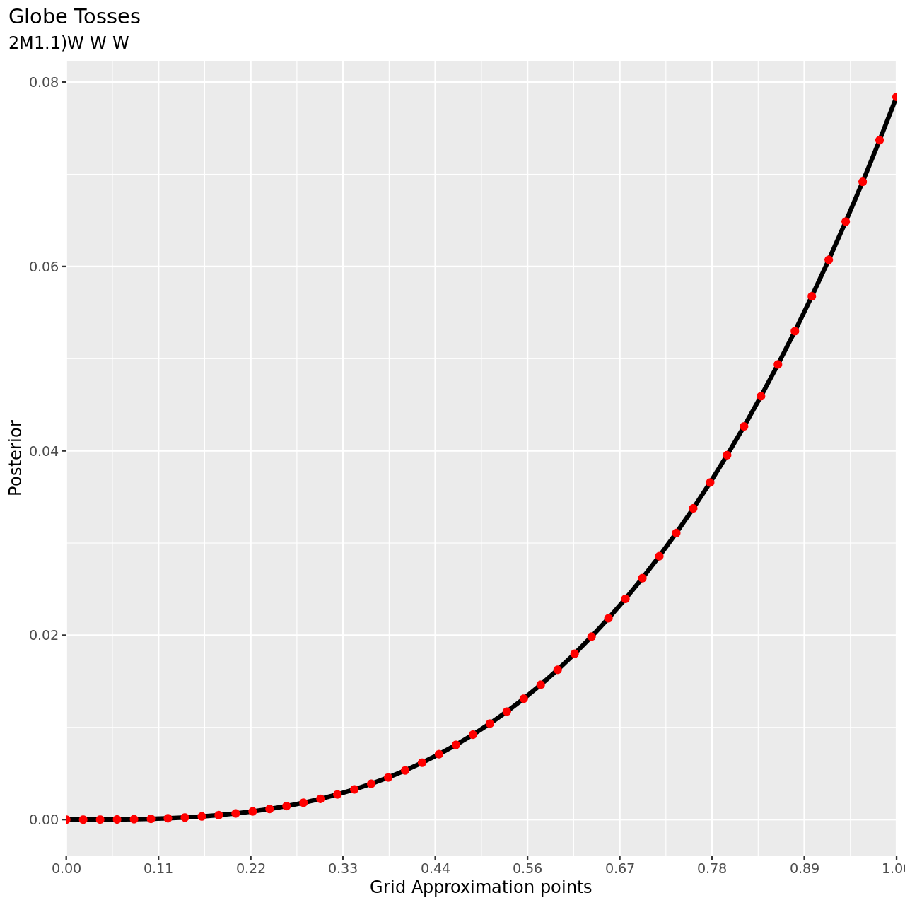
Recall the globe tossing model from the chapter. Compute and plot the grid approximate posterior distribution for each of the following sets of observations. In each case, assume a uniform prior for \(p\).
- W, W, W
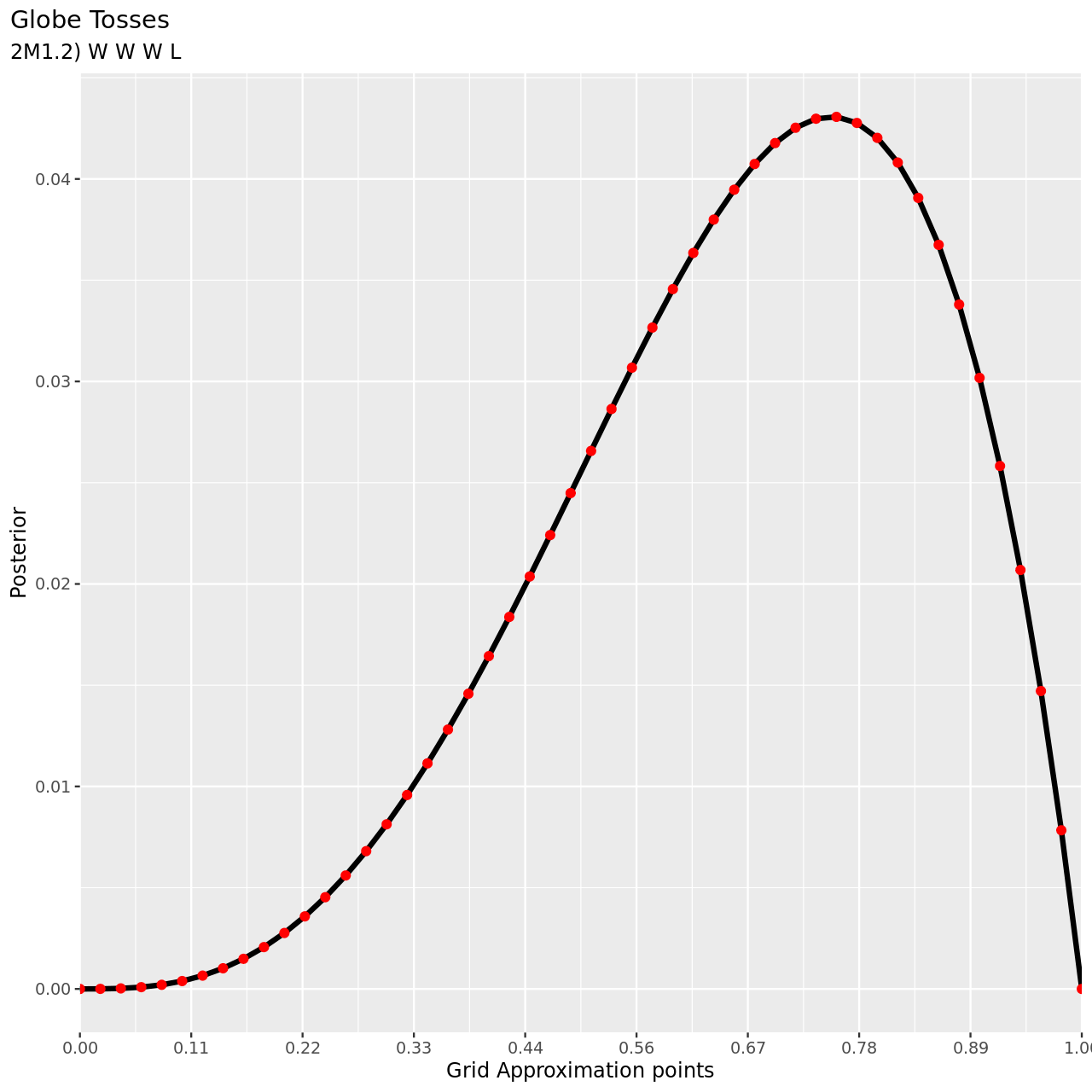
- W, W, W, L
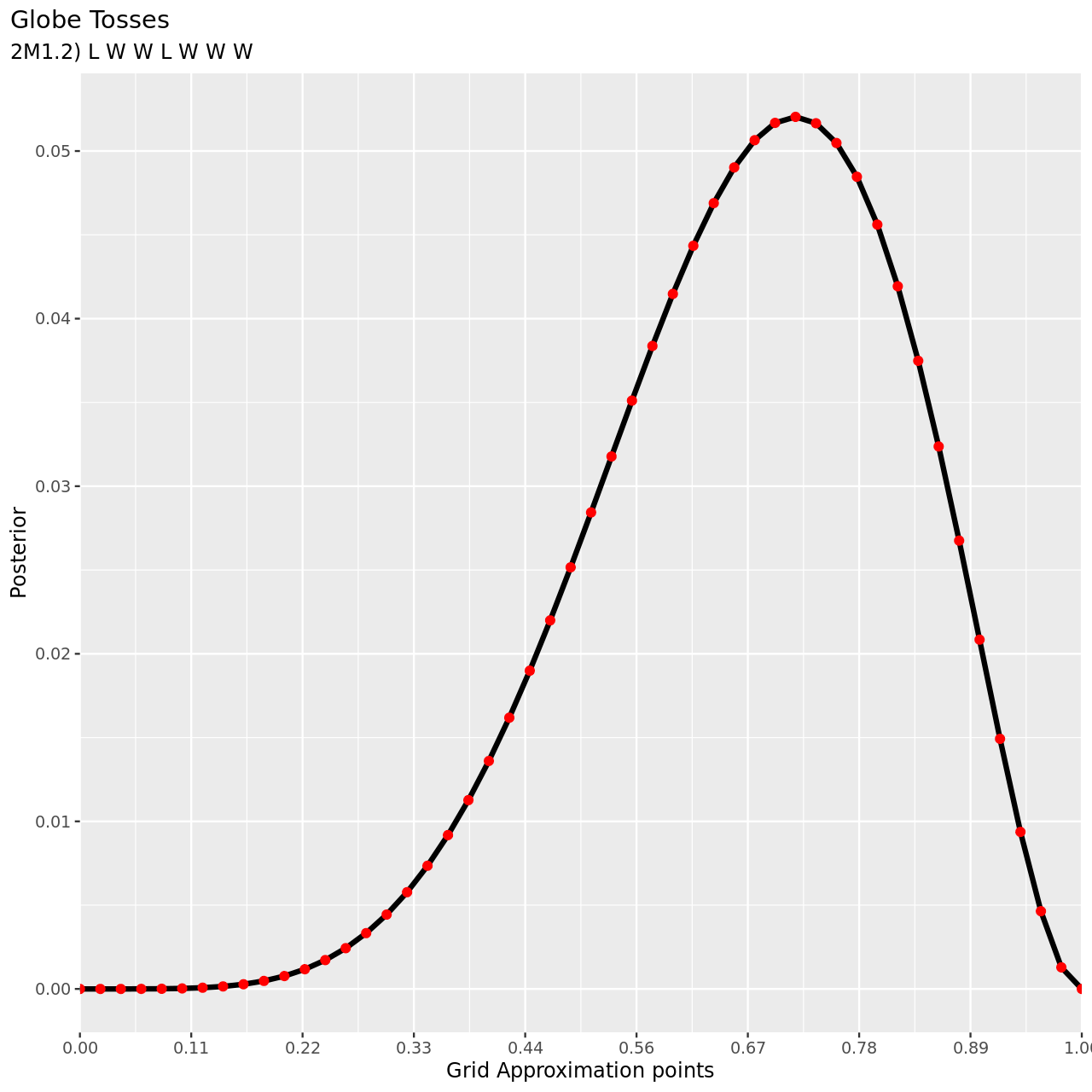
- L, W, W, L, W, W, W
Solution
 1nPoints<-50
 2# Grid
 3pGrid<-seq(0,1,length.out=nPoints)
 4# Prior
 5prior<-rep(1,nPoints)
 6# Likelihood for each grid point
 7likelihood<-pGrid %>% dbinom(3,3,prob=.)
 8noStdPosterior<-likelihood*prior
 9# Posterior
10posterior<- noStdPosterior / sum(noStdPosterior)
Now we can visualize this.
 1tibble(pGrid,posterior) %>% ggplot(aes(x=pGrid,y=posterior))+
 2  geom_line(size=3)+geom_point(size=5,color="red")+
 3  labs(
 4    title="Globe Tosses",
 5    subtitle="2M1.1)W W W",
 6    y="Posterior",
 7    x="Grid Approximation points"
 8  )+
 9  scale_x_continuous(breaks = seq(0,1,length.out=10),
10                     labels = seq(0,1,length.out=10) %>% sprintf("%.2f",.),
11                     expand = c(0, 0))+
12  theme(
13    plot.title.position = "plot",
14        )
For the remaining parts we will use a more abbreviated solution.
 1tibble(pGrid,
 2       li2=pGrid %>% dbinom(3,4,prob=.),
 3       prior) %>% mutate(post2unstd=li2*prior) %>% mutate(posterior=post2unstd/sum(post2unstd)) %>% ggplot(aes(x=pGrid,y=posterior))+
 4  geom_line(size=3)+geom_point(size=5,color="red")+
 5  labs(
 6    title="Globe Tosses",
 7    subtitle="2M1.2) W W W L",
 8    y="Posterior",
 9    x="Grid Approximation points"
10  )+
11  scale_x_continuous(breaks = seq(0,1,length.out=10),
12                     labels = seq(0,1,length.out=10) %>% sprintf("%.2f",.),
13                     expand = c(0, 0))+
14  theme(
15    plot.title.position = "plot"
16        )
For the final part, note that since the observations are independent, the ordering is irrelevant.
 1tibble(pGrid,
 2       li2=pGrid %>% dbinom(5,7,prob=.),
 3       prior) %>% mutate(post2unstd=li2*prior) %>% mutate(posterior=post2unstd/sum(post2unstd)) %>% ggplot(aes(x=pGrid,y=posterior))+
 4  geom_line(size=3)+geom_point(size=5,color="red")+
 5  labs(
 6    title="Globe Tosses",
 7    subtitle="2M1.2) L W W L W W W",
 8    y="Posterior",
 9    x="Grid Approximation points"
10  )+
11  scale_x_continuous(breaks = seq(0,1,length.out=10),
12                     labels = seq(0,1,length.out=10) %>% sprintf("%.2f",.),
13                     expand = c(0, 0))+
14  theme(
15    plot.title.position = "plot"
16        )
2M2
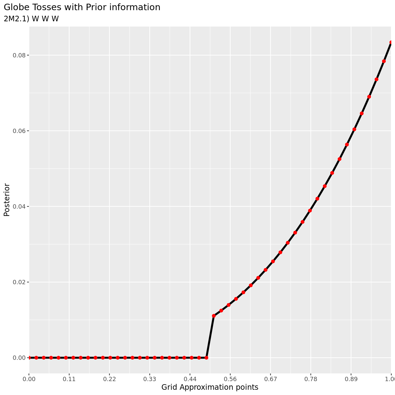
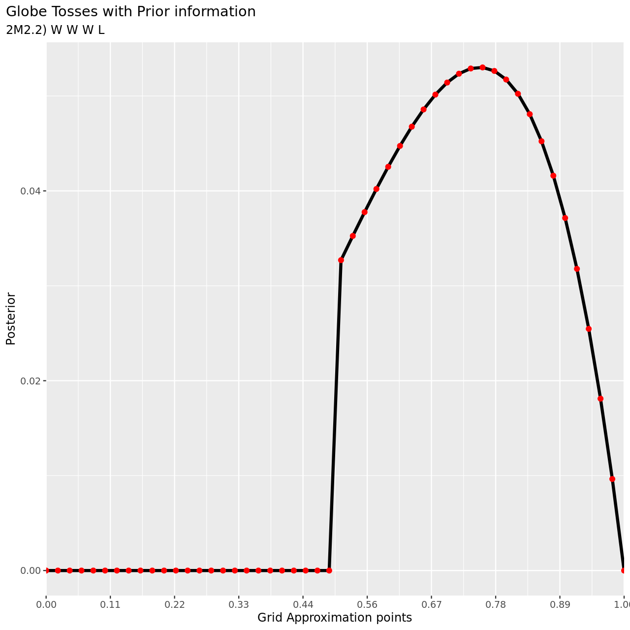
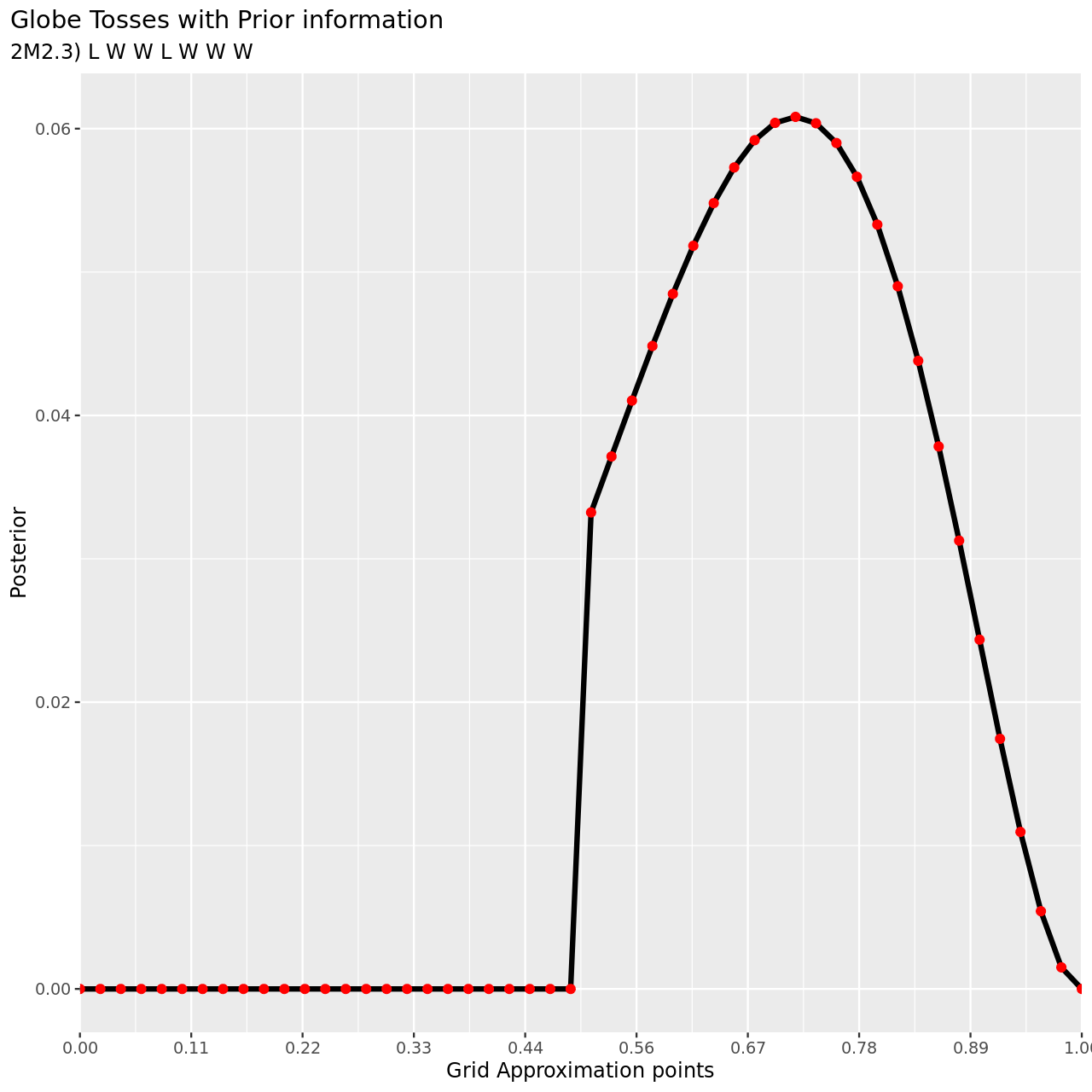
Now assume a prior for \(p\) that is equal to zero when \(p < 0.5\) and is a positive constant when \(p\geq 0.5\). Again compute and plot the grid approximate posterior distribution for each of the sets of observations in the problem just above.
- W, W, W
- W, W, W, L
- L, W, W, L, W, W, W
Solution
We proceed in much the same way as in the previous question. We also use the vectorized ifelse instead of explicitly using a for loop.
1nPoints<-50
2## Grid
3pGrid<-seq(0,1,length.out=nPoints)
4## Prior
5prior<-ifelse(pGrid<0.5,0,1)
 1tibble(pGrid,
 2       li2=pGrid %>% dbinom(3,3,prob=.),
 3       prior) %>% mutate(post2unstd=li2*prior) %>% mutate(posterior=post2unstd/sum(post2unstd)) %>% ggplot(aes(x=pGrid,y=posterior))+
 4  geom_line(size=3)+geom_point(size=5,color="red")+
 5  labs(
 6    title="Globe Tosses with Prior information",
 7    subtitle="2M2.1) W W W",
 8    y="Posterior",
 9    x="Grid Approximation points"
10  )+
11  scale_x_continuous(breaks = seq(0,1,length.out=10),
12                     labels = seq(0,1,length.out=10) %>% sprintf("%.2f",.),
13                     expand = c(0, 0))+
14  theme(
15    plot.title.position = "plot"
16        )
 1tibble(pGrid,
 2       li2=pGrid %>% dbinom(3,4,prob=.),
 3       prior) %>% mutate(post2unstd=li2*prior) %>% mutate(posterior=post2unstd/sum(post2unstd)) %>% ggplot(aes(x=pGrid,y=posterior))+
 4  geom_line(size=3)+geom_point(size=5,color="red")+
 5  labs(
 6    title="Globe Tosses with Prior information",
 7    subtitle="2M2.2) W W W L",
 8    y="Posterior",
 9    x="Grid Approximation points"
10  )+
11  scale_x_continuous(breaks = seq(0,1,length.out=10),
12                     labels = seq(0,1,length.out=10) %>% sprintf("%.2f",.),
13                     expand = c(0, 0))+
14  theme(
15    plot.title.position = "plot"
16        )
 1tibble(pGrid,
 2       li2=pGrid %>% dbinom(5,7,prob=.),
 3       prior) %>% mutate(post2unstd=li2*prior) %>% mutate(posterior=post2unstd/sum(post2unstd)) %>% ggplot(aes(x=pGrid,y=posterior))+
 4  geom_line(size=3)+geom_point(size=5,color="red")+
 5  labs(
 6    title="Globe Tosses with Prior information",
 7    subtitle="2M2.3) L W W L W W W",
 8    y="Posterior",
 9    x="Grid Approximation points"
10  )+
11  scale_x_continuous(breaks = seq(0,1,length.out=10),
12                     labels = seq(0,1,length.out=10) %>% sprintf("%.2f",.),
13                     expand = c(0, 0))+
14  theme(
15    plot.title.position = "plot"
16        )
2M4
Suppose you have a deck with only three cards. Each card has two sides, and each side is either black or white. One card has two black sides. The second card has one black and one white side. The third card has two white sides. Now suppose all three cards are placed in a bag and shuffled. Someone reaches into the bag and pulls out a card and places it flat on a table. A black side is shown facing up, but you don’t know the color of the side facing down. Show that the probability that the other side is also black is 2/3. Use the counting method (Section 2 of this chapter) to approach this problem. This means counting up the ways that each card could produce the observed data (a black side facing up on the table).
Solution
Let us begin by defining what is given to us.
- There are three cards
- One has a black side and a white side (cBW)
- One is colored black on both sides (cBB)
- One is colored white on both sides (cWW)
Our total probability universe is defined by all possible states defined by the enumeration of possible states for each card and their combinations. In other words, it is a universe defined by color and the number of cards.
The question posed is essentially, given a single observation, that is that a random draw from our universe has produced a black side (note that we already know that there is one card so it satisfies the requirements of being a valid state of the universe we are considering), what is the probability of the other side being black as well?
Hence we can express this as O: cB? and we need P(B|cB?). We will enumerate possibilities of observing the black side in our universe.
- cBW
- This has \(1\) way of producing cB?
- cBB
- This has \(2\) ways of producing cB?
- cWW
- This has \(0\) ways of producing cB?
| Card | Ways to cB? |
|---|---|
| cBW | 1 |
| cBB | 2 |
| cWW | 0 |
So we see that there are \(3\) ways to see a black side in a single draw, and two of these come from (cBB), thus the probability of seeing another black side is \(\frac{2}{3}\).
Chapter III: Sampling the Imaginary
Easy Questions (Ch3)
These questions are associated with the following code snippet for the globe tossing example.
1p_grid<-seq(from=0, to=1, length.out=1000)
2prior<-rep(1,1000)
3likelihood<-dbinom(6,size=9,prob=p_grid)
4posterior<-likelihood*prior
5posterior<-posterior/sum(posterior)
6set.seed(100)
7samples<-sample(p_grid,prob=posterior,size=1e4,replace=TRUE)
3E1
How much posterior probability lies below \(p = 0.2\)?
Solution
We can check the number of samples as follows:
1ifelse(samples<0.2,1,0) %>% sum(.)
1[1] 4
Now we will simply divide by the number of samples.
1ifelse(samples<0.2,1,0) %>% sum(.)/1e4
1[1] 4e-04
More practically, the percentage of the probability density below \(p=0.2\) is:
1ifelse(samples<0.2,1,0) %>% sum(.)/1e4 *100
1[1] 0.04
3E2
How much posterior probability lies above \(p = 0.8\)?
Solution
1ifelse(samples>0.8,1,0) %>% sum(.)/1e4 *100
1[1] 11.16
3E3
How much posterior probability lies between \(p = 0.2\) and \(p = 0.8\)?
Solution
1ifelse(samples>0.2 & samples<0.8,1,0) %>% sum(.)/1e4 *100
1[1] 88.8
3E4
20% of the posterior probability lies below which value of \(p\)?
Solution
1samples %>% quantile(0.2)
1      20%
20.5185185
3E5
20% of the posterior probability lies above which value of \(p\)?
Solution
1samples %>% quantile(0.8)
1      80%
20.7557558
Questions of Medium Complexity (Ch3)
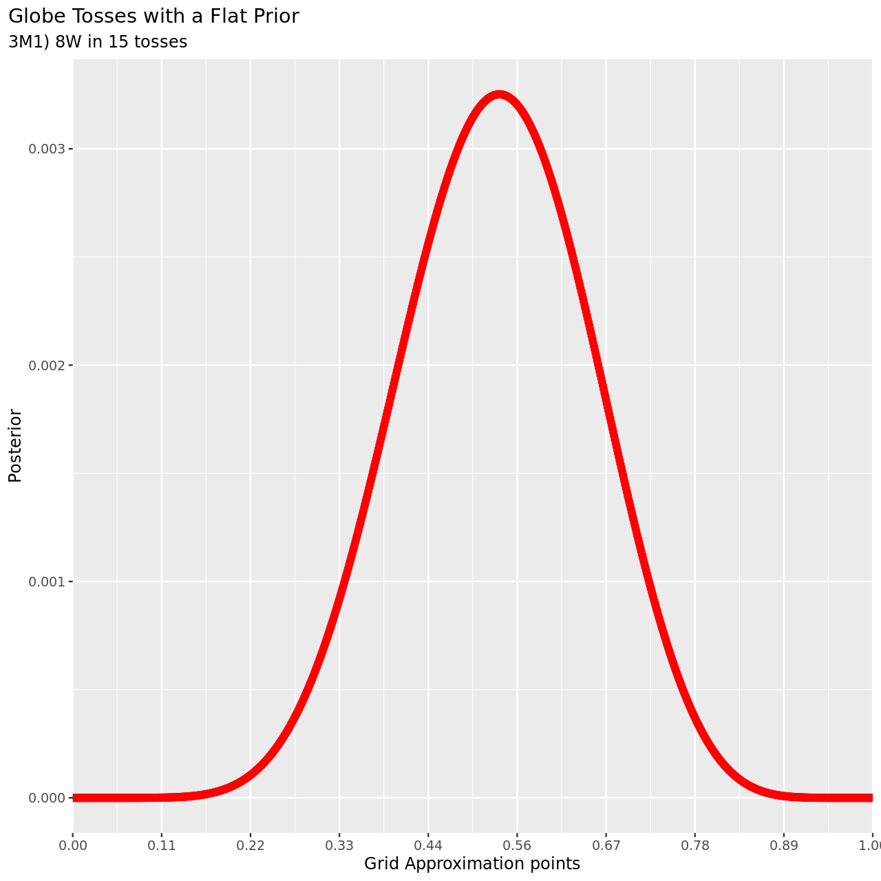
3M1
Suppose the globe tossing data had turned out to be 8 water in 15 tosses. Construct the posterior distribution, using grid approximation. Use the same flat prior as before.
Solution
1nPoints<-1000
2## Grid
3pGrid<-seq(0,1,length.out=nPoints)
4## Prior
5prior<-rep(1,nPoints)
 1tibble(pGrid,
 2       li2=pGrid %>% dbinom(8,15,prob=.),
 3       prior) %>% mutate(post2unstd=li2*prior) %>% mutate(posterior=post2unstd/sum(post2unstd)) %>% ggplot(aes(x=pGrid,y=posterior))+
 4  geom_line(size=3)+geom_point(size=5,color="red")+
 5  labs(
 6    title="Globe Tosses with a Flat Prior",
 7    subtitle="3M1) 8W in 15 tosses",
 8    y="Posterior",
 9    x="Grid Approximation points"
10  )+
11  scale_x_continuous(breaks = seq(0,1,length.out=10),
12                     labels = seq(0,1,length.out=10) %>% sprintf("%.2f",.),
13                     expand = c(0, 0))+
14  theme(
15    plot.title.position = "plot"
16        )
3M2
Draw 10,000 samples from the grid approximation from above. Then use the samples to calculate the 90% HPDI for \(p\).
Solution
For this, we will create a tibble of the experiment and then sample from it.
1exp3m2<-tibble(pGrid,
2       li2=pGrid %>% dbinom(8,15,prob=.),
3       prior) %>% mutate(post2unstd=li2*prior) %>% mutate(posterior=post2unstd/sum(post2unstd))
4
5sample(pGrid,prob=exp3m2$posterior,size=1e4,replace=TRUE) %>% HPDI(prob=0.9)
1
2     |0.9      0.9|
30.3293293 0.7167167
3M3
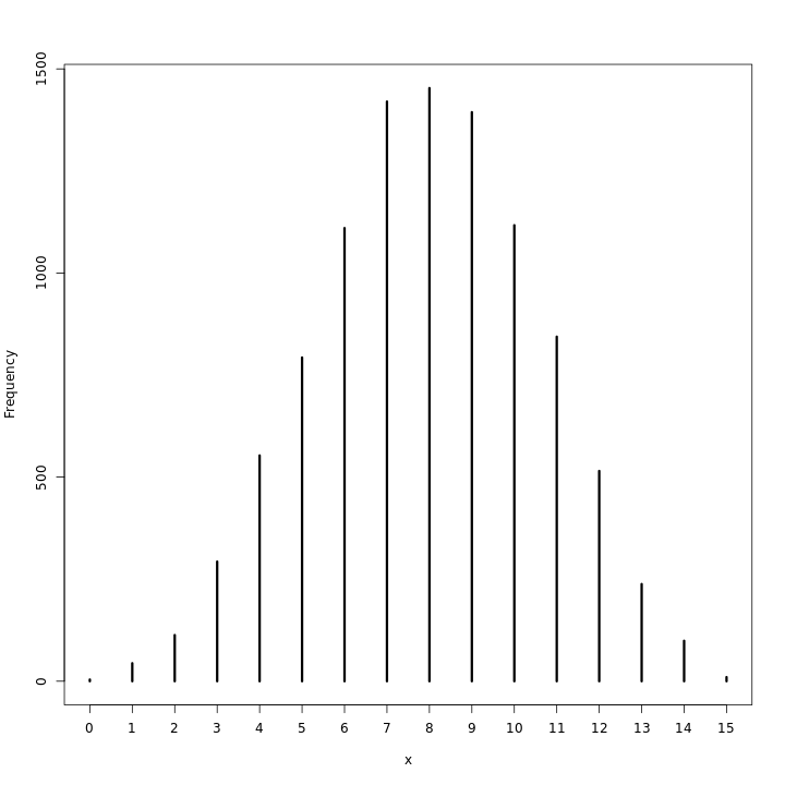
Construct a posterior predictive check for this model and data. This means simulate the distribution of samples, averaging over the posterior uncertainty in \(p\). What is the probability of observing 8 water in 15 tosses.
Solution
As covered in the chapter, we will sample from the posterior distribution and
use that to obtain experiment instances with rbinom. Finally we will then use
these instances to count our way to the probability of observing the true data.
1waterPred<-sample(pGrid,prob=exp3m2$posterior,size=1e4,replace=TRUE) %>% rbinom(1e4,size=15,prob=.)
2ifelse(waterPred==8,1,0) %>% sum(.)/1e4
1[1] 0.1447
This seems like a very poor model, but the spread of the realizations is probably a better measure.
1waterPred %>% summary
1   Min. 1st Qu.  Median    Mean 3rd Qu.    Max.
2  0.000   6.000   8.000   7.936  10.000  15.000
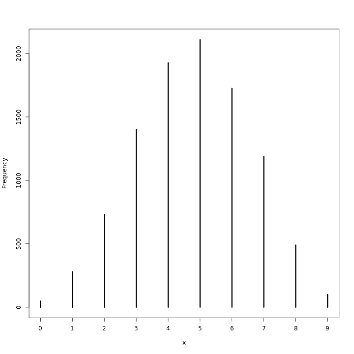
This does seem to indicate that at any rate the realizations are close enough to 8 for the model to be viable. A visualization of this should also be checked.
1waterPred %>% simplehist
3M4
Using the posterior distribution constructed from the new (8/15) data, now calculate the probability of observing 6 water in 9 tosses
Solution
We will reuse the posterior, and recalculate our samples (corresponding to new possible instances).
1waterPred<-sample(pGrid,prob=exp3m2$posterior,size=1e4,replace=TRUE) %>% rbinom(1e4,size=9,prob=.)
1ifelse(waterPred==6,1,0) %>% sum(.)/1e4
2waterPred %>% summary
1[1] 0.1723
2
3   Min. 1st Qu.  Median    Mean 3rd Qu.    Max.
4  0.000   4.000   5.000   4.777   6.000   9.000
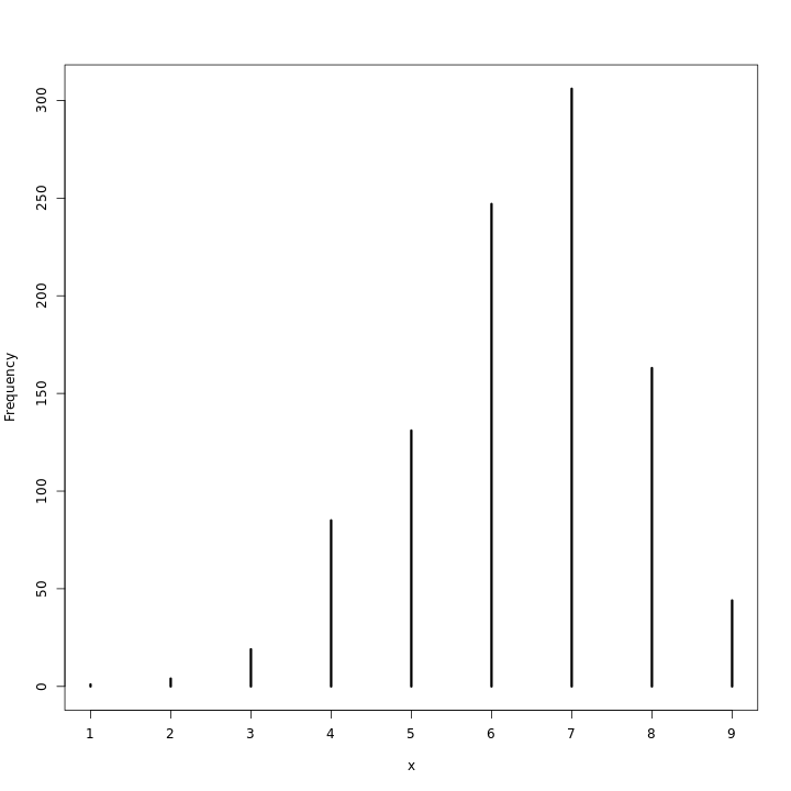
Though the numerical value is not very different from the previous solution, we note that the centrality measures are much worse.
1waterPred %>% simplehist
3M6
Suppose you want to estimate the Earth’s proportion of water very precisely. Specifically, you want the 99% percentile interval of the posterior distribution of p to be only 0.05 wide. This means the distance between the upper and lower bound of the interval should be 0.05. How many times will you have to toss the globe to do this?
Solution
Since the no information of the model has been provided here, we will consider reason out an approach, before making an estimate.
The number globe tosses corresponds to the number of observations we require. A percentile interval this narrow will essentially require a large number of samples i.e. be in the large number limit, so the choice of prior should not matter much. The width of our interval should also be related to the number of grid points we use in our approximation.
We will first use the true amount of water on the planet (approximately 71 percent) to generate information for the number of throws.
Let us generate observations.
1nThrows<-10000
2nWater<-0.71*nThrows %>% round
We will set up a simple model for this, with an indifferent prior along with a better prior.
1nPoints<-1000
2## Grid
3pGrid<-seq(0,1,length.out=nPoints)
4## Prior
5prior<-rep(1,nPoints)
6betterPrior<-ifelse(pGrid<0.5,0,1)
We will define a function for generating our results since we will need to perform this a few times.
 1genModel<- function(nThrows){
 2nWater<-0.71*nThrows %>% round
 3tibble(pGrid,
 4       li2=pGrid %>% dbinom(nWater,nThrows,prob=.),
 5       prior,betterPrior) %>%
 6  mutate(
 7    postUnifNSD=li2*prior,
 8    postUnif=postUnifNSD/sum(postUnifNSD),
 9    smplUnif=sample(pGrid,
10                    prob=postUnif,
11                    size=nrow(.),
12                    replace=TRUE),
13    predUnif=rbinom(nrow(.),size=9,prob=smplUnif),
14    postBPNSD=li2*betterPrior,
15    postBP=postBPNSD/sum(postBPNSD),
16    smplBP=sample(pGrid,
17                    prob=postBP,
18                    size=nrow(.),
19                    replace=TRUE),
20    predBP=rbinom(nrow(.),size=9,prob=smplBP)
21  )
22}
It would be nice to look at the different priors as well.
1genModel2(1e4) %>% .$predBP %>% simplehist
1genModel(1e6) %>% .$predUnif %>% simplehist
As can be expected, with the large number of observations, the priors barely make a difference.
We note that what we are looking for is a credibility width of less than 0.05 at a probability of 0.99.
1get99Width<- function(x,nx) {
2  piInter<-PI(x$postUnif,prob=0.99)
3  hpdiInter<-HPDI(x$postUnif,prob=0.99)
4  tibble(wPI=piInter[2]-piInter[1],wHPDI=hpdiInter[2]-hpdiInter[1],nSamples=nx)
5}
Now we are in a position to start testing samples.
1base100<-genModel(1e2) %>% get99Width(1e2)
2t<-1000
3while(min(base100$wPI) & min(base100$wHPDI) > 0.005) {
4  t<-t*10
5  base100<-genModel(t) %>% get99Width(t) %>% bind_rows(base100)
6}
7base100 %>% toOrg
1
2|                 wPI |               wHPDI | nSamples |
3|---------------------+---------------------+----------|
4|  0.0464554168997065 | 0.00121611594937107 |    1e+05 |
5|  0.0735809517149284 |  0.0511200696528017 |    10000 |
6| 0.00884431494702241 |  0.0088121623437198 |      100 |
There is an inherent problem with this formulation, and that is that the model confidence is based on the observations which were drawn to emulate the true distribution of water on Earth. This means that a highly tight width, should be recognized to still be highly dependent on the observed data. Let us try to obtain the same intervals with a randomized observation setup instead.
In order to do this we simply modify the number of water observations.
 1genModel2<- function(nThrows){
 2tibble(pGrid,
 3       li2=pGrid %>% dbinom(sample(1:nThrows, 1, replace=TRUE),nThrows,prob=.),
 4       prior,betterPrior) %>%
 5  mutate(
 6    postUnifNSD=li2*prior,
 7    postUnif=postUnifNSD/sum(postUnifNSD),
 8    smplUnif=sample(pGrid,
 9                    prob=postUnif,
10                    size=nrow(.),
11                    replace=TRUE),
12    predUnif=rbinom(nrow(.),size=9,prob=smplUnif),
13    postBPNSD=li2*betterPrior,
14    postBP=postBPNSD/sum(postBPNSD),
15    smplBP=sample(pGrid,
16                    prob=postBP,
17                    size=nrow(.),
18                    replace=TRUE),
19    predBP=rbinom(nrow(.),size=9,prob=smplBP)
20  )
21}
We can now test these the same way.
1base100<-genModel2(100) %>% get99Width(100)
2t<-100
3while(min(base100$wPI) & min(base100$wHPDI) > 0.05) {
4  t<-t+100
5  base100<-genModel2(t) %>% get99Width(t) %>% bind_rows(base100)
6}
7base100 %>% toOrg
1
2|                 wPI |               wHPDI | nSamples |
3|---------------------+---------------------+----------|
4| 0.00853874459759265 | 0.00851020493831213 |      100 |
Chapter IV: Geocentric Models
Easy Questions (Ch4)
4E1
In the model definition below, which line is the likelihood?
Solution
The likelihood is defined by the first line, that is, \(y_i \sim\mathrm{Normal}(\mu, \sigma)\)
4E2
In the model definition above, how many parameters are in the posterior distribution?
Solution
The model has two parameters for the posterior distribution, \(\mu\) and \(\sigma\).
4E3
Using the model definition above, write down the appropriate form of Bayes’ theorem that includes the proper likelihood and priors.
Solution
The appropriate form of Bayes’ theorem in this case is:
\[ \mathrm(Pr)(\mu,\sigma|y)=\frac{\mathrm{Normal}(y|\mu,\sigma)\mathrm{Normal}(\mu|0,10)\mathrm{Exponential}(\sigma|1)}{\int\int \mathrm{Normal}(y|\mu,\sigma)\mathrm{Normal}(\mu|0,10)\mathrm{Exponential}(\sigma|1)d\mu d\sigma} \]
4E4
In the model definition below, which line is the linear model?
Solution
The second line is the linear model in the definition, that is: \[\mu_i = \alpha + \beta x_i\]
4E5
In the model definition just above, how many parameters are in the posterior distribution?
Solution
The model defined has three independent parameters for the posterior distribution, which are \(\alpha\), \(\beta\) and \(\sigma\). Though \(\mu\) is a parameter, it is defined in terms of \(\alpha\), \(\beta\) and \(x\) so will not be considered to be a parameter for the posterior.
Questions of Medium Complexity (Ch4)
4M1
For the model definition below, simulate observed \(y\) values from the prior (not the posterior).
Solution
Sampling from the prior involves averaging over the prior distributions of \(\mu\) and \(\sigma\).
1muPrior<-rnorm(1e4,0,10)
2sigmaPrior<-rexp(1e4,1)
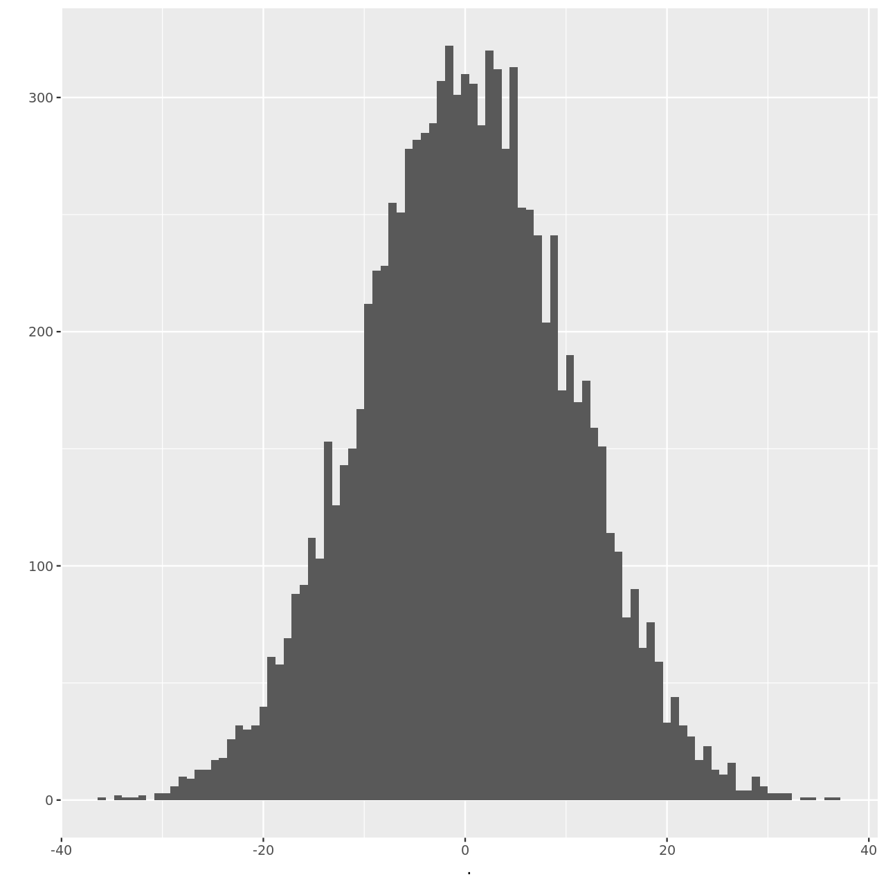
3hSim<-rnorm(1e4,muPrior,sigmaPrior)
We can visualize this as well.
1hSim %>% qplot(binwidth=0.8)
4M2
Translate the model just above into a quap formula.
Solution
1ex4m2<-alist(
2  y~dnorm(mu,sigma),
3  mu~dnorm(0,10),
4  sigma~dexp(1)
5)
4M3
Translate the quap model formula below into a mathematical model
definition
Solution
The model defined can be expressed mathematically as:
4M4
A sample of students is measured for height each year for 3y ears. After the third year,you want to fit a linear regression predicting height using year as a predictor. Write down the mathematical model definition for this regression, using any variable names and priors you choose. Be prepared to defend your choice of priors.
Solution
Let us first declare a model.
Where the double subscript is meant to indicate that the data is obtained both per year and per student. That is, we have:
- \(y_{ij}\) is the height of each student each year
- \(x_{j}\) is the “reduced” year, that is the difference between a particular year and the average sample year
The prior distributions are not too complicated. Since the distribution of males and females in the student population is missing, as is information on the age distribution, we will set a conservative lower value of 120 centimeters, based on the understanding that the students have at-least 3 years in school, so they are growing, so we assume students grow around 8 centimeters every year.
The distribution for beta is a log-normal distribution to ensure that we do not sample negative values which might arise from sampling a Gaussian. This is due to the assumption that the students grow every year.
Following the procedures of the chapter, we will visualize realizations from the prior.
1nDraws<-50
2a<-rnorm(nDraws,100,8)
3b<-rlnorm(nDraws,0,2)
4sigmaPrior<-rexp(nDraws,1)
We will express our yearly function:
1genYr<- function(x,yr) {rnorm(1,a[x]+b[x]*(yr-1.5),sigmaPrior[x])}
Now we will assume a class size of 35 for our priors.
1testDat<-tibble(student=1:36)
2testDat$year1<-sapply(testDat$student,FUN=genYr,yr=1)
3testDat$year2<-sapply(testDat$student,FUN=genYr,yr=2)
4testDat$year3<-sapply(testDat$student,FUN=genYr,yr=3)
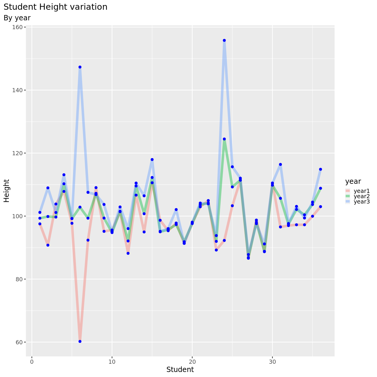
We will now look at this.
 1testDat %>% pivot_longer(-student,names_to = "year",values_to = "height") %>% ggplot(aes(x=student,y=height,color=year))+
 2  geom_line(size=4,alpha=0.4)+
 3  geom_point(size=4,colour="blue")+
 4  labs(
 5    title="Student Height variation",
 6    subtitle="By year",
 7    y="Height",
 8    x="Student"
 9  )+
10  theme(
11    plot.title.position = "plot",
12        )
 1testDat %>% pivot_longer(-student,names_to = "year",values_to = "height") %>% ggplot(aes(x=year,y=height,color=student))+
 2  geom_line(size=4,alpha=0.4)+
 3  geom_point(size=4,colour="blue")+
 4  labs(
 5    title="Student Height variation",
 6    subtitle="By year",
 7    y="Height",
 8    x="Student"
 9  )+
10  theme(
11    plot.title.position = "plot",
12        )
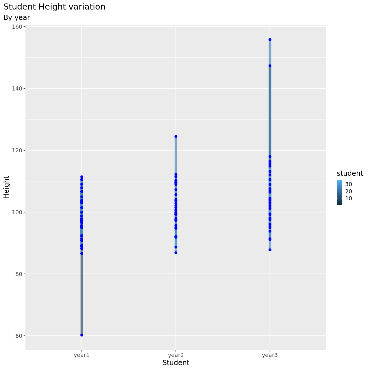
This seems to be a pretty reasonable model, all things considered.
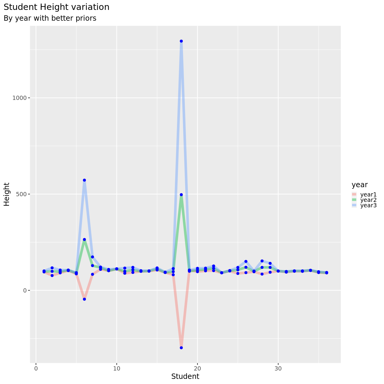
4M5
Now suppose I remind you that every student got taller each year. Does this information lead you to change your choice of priors? How?
Solution
Since we have incorporated a LogNormal term, we do not need to change our choice of prior. However, the parameters of our previous model did include some heights decreasing, so we will modify the LogNormal distribution on beta. Recall that we would like to see around 7 centimeters of growth, so our mean should be exp(1+2/2) which is around 7.
Simulating draws as before.
1nDraws<-50
2a<-rnorm(nDraws,100,8)
3b<-rlnorm(nDraws,1,2)
4sigmaPrior<-rexp(nDraws,1)
5genYr<- function(x,yr) {rnorm(1,a[x]+b[x]*(yr-1.5),sigmaPrior[x])}
6testDat<-tibble(student=1:36)
7testDat$year1<-sapply(testDat$student,FUN=genYr,yr=1)
8testDat$year2<-sapply(testDat$student,FUN=genYr,yr=2)
9testDat$year3<-sapply(testDat$student,FUN=genYr,yr=3)
 1testDat %>% pivot_longer(-student,names_to = "year",values_to = "height") %>% ggplot(aes(x=student,y=height,color=year))+
 2  geom_line(size=4,alpha=0.4)+
 3  geom_point(size=4,colour="blue")+
 4  labs(
 5    title="Student Height variation",
 6    subtitle="By year with better priors",
 7    y="Height",
 8    x="Student"
 9  )+
10  theme(
11    plot.title.position = "plot",
12        )
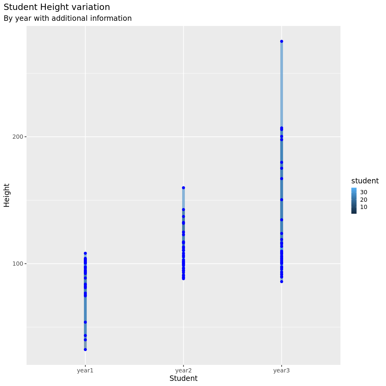
4M6
Now suppose I tell you that the variance among heights for students of the same age is never more than 64cm. How does this lead you to revise your priors?
Solution
This information will change the variance term in our model. We will incorporate this into our model by using a uniform distribution for sigma. The new model is then:
Simulating draws as before.
1nDraws<-50
2a<-rnorm(nDraws,100,8)
3b<-rlnorm(nDraws,1,2)
4sigmaPrior<-runif(nDraws,0,8)
5genYr<- function(x,yr) {rnorm(1,a[x]+b[x]*(yr-1.5),sigmaPrior[x])}
6testDat<-tibble(student=1:36)
7testDat$year1<-sapply(testDat$student,FUN=genYr,yr=1)
8testDat$year2<-sapply(testDat$student,FUN=genYr,yr=2)
9testDat$year3<-sapply(testDat$student,FUN=genYr,yr=3)
We will now look at this.
 1testDat %>% pivot_longer(-student,names_to = "year",values_to = "height") %>% ggplot(aes(x=year,y=height,color=student))+
 2  geom_line(size=4,alpha=0.4)+
 3  geom_point(size=4,colour="blue")+
 4  labs(
 5    title="Student Height variation",
 6    subtitle="By year with additional information",
 7    y="Height",
 8    x="Student"
 9  )+
10  theme(
11    plot.title.position = "plot",
12        )
 1testDat %>% pivot_longer(-student,names_to = "year",values_to = "height") %>% mutate(year=year %>% as.factor %>% as.numeric) %>% filter(student==3) %>% ggplot(aes(x=year,y=height,color=student))+
 2  geom_line(size=4,alpha=0.4)+
 3  geom_point(size=4,colour="blue")+
 4  labs(
 5    title="Student Height variation with additional information",
 6    subtitle="By year",
 7    y="Height",
 8    x="year"
 9  )+
10  theme(
11    plot.title.position = "plot",
12        )
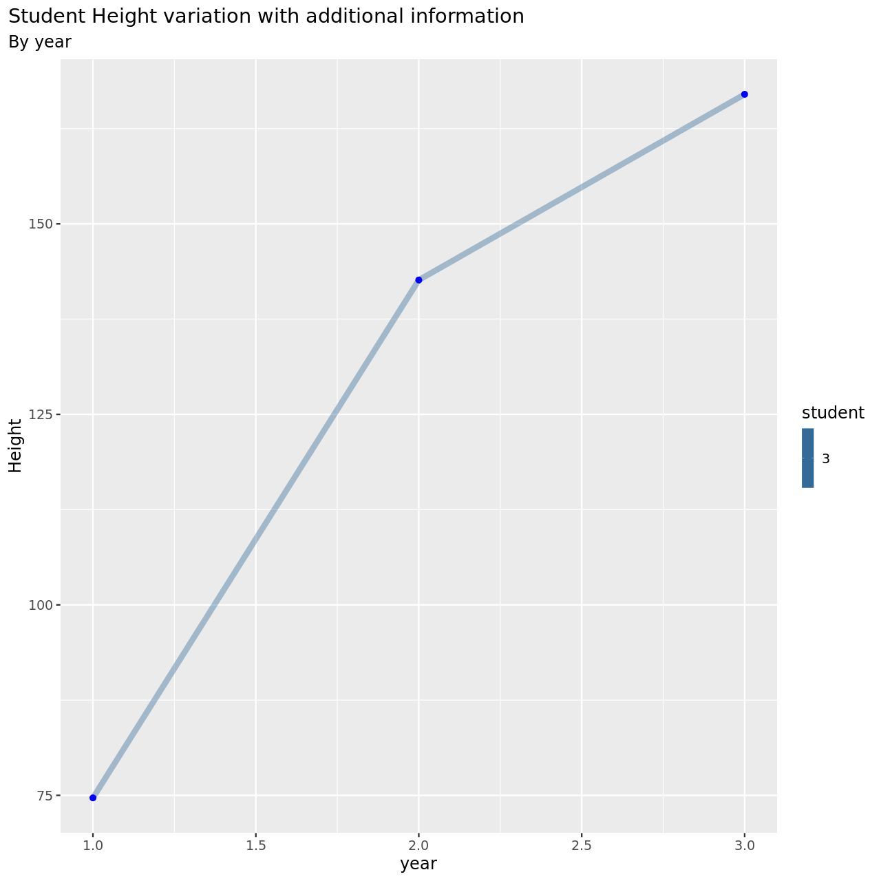 This is now much more reasonable.
4M7
Refit model m4.3 from the chapter, but omit the mean weight xbar
this time. Compare the new model’s posterior to that of the original
model. In particular, look at the covariance among the parameters. What
is different? Then compare the posterior predictions of both models.
Solution
Let us re-create the original data model first.
1data(Howell1)
2howDat<-Howell1
3howDat<-howDat %>% filter(age>=18)
Recall that the original model was given by:
 1xbar<-mean(howDat$weight)
 2m43<-quap(
 3  alist(
 4    height ~ dnorm(mu,sigma),
 5    mu<-a+b*(weight-xbar),
 6    a ~ dnorm(178,20),
 7    b ~ dlnorm(0,1),
 8    sigma ~ dunif(0,50)
 9  ),data=howDat
10)
11m43 %>% precis %>% toOrg
| row.names | mean | sd | 5.5% | 94.5% |
|---|---|---|---|---|
| a | 154.601366268055 | 0.270307670586024 | 154.169362403256 | 155.033370132855 |
| b | 0.90328084058895 | 0.041923632631821 | 0.83627877851613 | 0.970282902661771 |
| sigma | 5.07188106954248 | 0.191154797986941 | 4.76637878273641 | 5.37738335634854 |
Now we can incorporate the new information we have.
 1m43b<-quap(
 2  alist(
 3    height ~ dnorm(mu,sigma),
 4    mu<-a+b*weight,
 5    a ~ dnorm(178,20),
 6    b ~ dlnorm(0,1),
 7    sigma ~ dunif(0,50)
 8  ),data=howDat
 9)
10m43b %>% precis %>% toOrg
| row.names | mean | sd | 5.5% | 94.5% |
|---|---|---|---|---|
| a | 114.515009160638 | 1.89397291870405 | 111.488074634765 | 117.54194368651 |
| b | 0.891112682994587 | 0.0416750085549524 | 0.824507970215838 | 0.957717395773337 |
| sigma | 5.06263423083996 | 0.190299406826185 | 4.75849902431897 | 5.36676943736095 |
Thus we note that the slope is the same, while the intercept changes. Now we need to check the covariances. We will convert from the variable covariance scale to the correlation matrix.
1m43b %>% vcov %>% cov2cor %>% round(.,2)
1          a     b sigma
2a      1.00 -0.99  0.02
3b     -0.99  1.00 -0.02
4sigma  0.02 -0.02  1.00
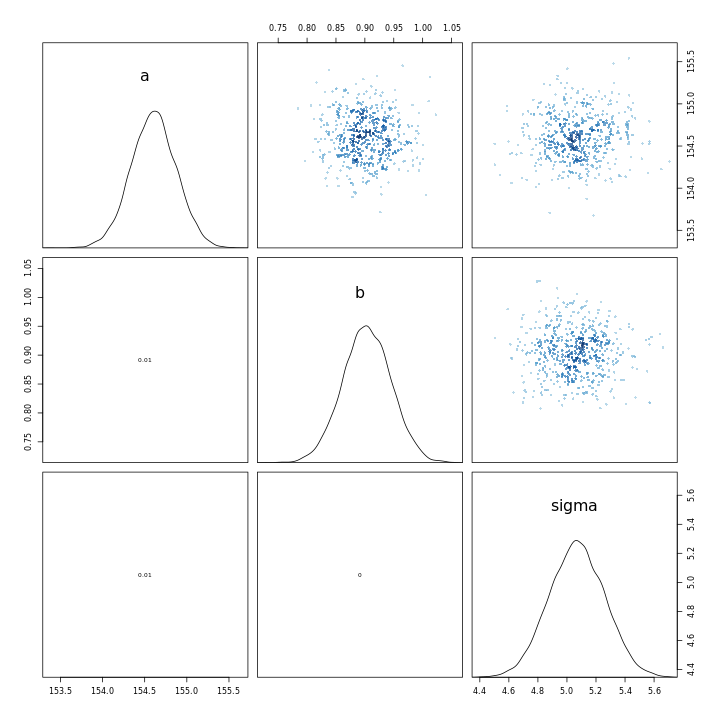
1m43 %>% vcov %>% cov2cor %>% round(.,2)
1      a b sigma
2a     1 0     0
3b     0 1     0
4sigma 0 0     1
The contrast between the two is very clear from the correlation matrices, the new model has an almost perfect negatively correlated intercept and slope.
1m43 %>% pairs
1m43b %>% pairs
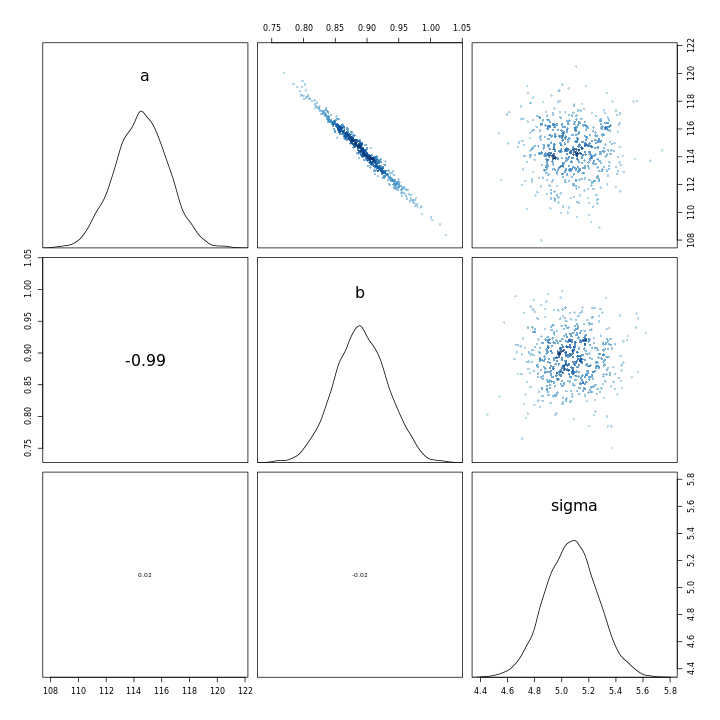
This indicates that the scaling of the variables leads to a completely different model in terms of the parameter relationships, in-spite of the fact that the models have almost the same posterior predictions.
Summer of 2020 ↩︎
![]()