
27 minutes
Written: 2020-06-14 00:00 +0000
Updated: 2020-08-18 23:28 +0000
SR2 :: Solutions for Chapters {5,6,7}
Setup details are described here, and the meta-post about these solutions is here.
Materials
The summmer course1 is based off of the second edition of Statistical Rethinking by Richard McElreath. This post covers the following exercise questions:
- Chapter 5
- E{1,2,3,4}
- M{1,2,3,5}
- Chapter 6
- E{1,2,3,4}
- M{1,2,3}
- Chapter 7
- E{1,2,3,4}
- M{1,2,3,4,5,6}
Packages
A colophon with details is provided at the end, but the following packages and theme parameters are used throughout.
1libsUsed<-c("tidyverse","tidybayes","orgutils","dagitty",
2            "rethinking","tidybayes.rethinking",
3            "ggplot2","kableExtra","dplyr","glue",
4            "latex2exp","data.table","printr","devtools")
5invisible(lapply(libsUsed, library, character.only = TRUE));
6theme_set(theme_grey(base_size=24))
Chapter V: The Many Variables & The Spurious Waffles
Easy Questions (Ch5)
5E1
Which of the linear models below are multiple linear regressions?
- \(μᵢ=α+βxᵢ\)
- \(μᵢ=βₓxᵢ+β_{z}zᵢ\)
- \(μᵢ=α+β(xᵢ-zᵢ)\)
- \(μᵢ=α+βₓxᵢ+β_{z}zᵢ\)
Solution
A multiple regression problem is one with more than one predictor and corresponding coefficients in an additive (hence “linear”) manner. By this logic, we can analyze the options as follows:
- Has one predictor variable, \(x\) thus is not a multiple regression
- Is a multiple linear regression since there are two independent variables, \(x\) and \(z\)
- Is not a multiple regression model, since only the difference of \(x\) and \(z\) enters the model (with slope \(\beta\))
- This is a multiple linear regression problem, since there are two predictor variables \(x\) and \(z\)
Thus options two and four are correct.
5E2
Write down a multiple regression to evaluate the claim: Animal diversity is linearly related to latitude, but only after controlling for plant diversity. You just need to write down the model definition.
Solution
Without any further information, we can simply write a model for diversity as:
\[D_{A}\sim\mathrm{Log-Normal}(μᵢ,σ)\] \[μᵢ=α+β_{L}Lᵢ+β_{D_P}D_{Pᵢ}\]
Where:
- \(D_{A}\) is the animal diversity
- \(D_{P}\) is the plant diversity
- \(L\) is the latitude
We have used a log-normal distribution for the animal diversity, since negative values for diversity are meaningless. This arises from the understanding that the diversity is on an ordinal scale with classes. The linear model posits a linear model which has two predictors, the latitude and plant diversity. Thus this model allows for “control” of the plant diversity.
Further details would be relegated to the choice of priors instead of the model.
5E3
Write down a multiple regression to evaluate the claim: Neither amount of funding nor size of laboratory is by itself a good predictor of time to PhD degree; but together these variables are both positively associated with time to degree. Write down the model definition and indicate which side of zero each slope parameter should be on.
Solution
Without considering priors, we would like to write a linear model with two variables, funding and the lab size. To allow for extensions later regarding the type of funding, we will use “money” and “time” as inputs for the model. Again, since the time to a PhD cannot be negative, we will posit a log-normal distribution.
\[Tᵢ∼\mathrm{Log-Normal}(μᵢ,σ)\] \[μᵢ=α+β_{M}M_{i}+β_{S}Sᵢ\]
Where:
- \(Tᵢ\) is the time to completion
- \(M\) corresponds to money
- \(S\) corresponds to the size of the lab
Since we are told that the variables considered jointly have a positive association with the time, we note that the slope parameters for both should be positive.
5E4
Suppose you have a single categorical predictor with 4 levels (unique values), labeled A,B,C and D. Let \(Aᵢ\) be an indicator variable that is \(1\) where case \(i\) is in category A. Also suppose \(Bᵢ\), \(Cᵢ\) and \(Dᵢ\) for the other categories. Now which of the following linear models are inferentially equivalent ways to include the categorical variable in a regression? Models are inferentially equivalent when it’s possible to compute one posterior distribution from the posterior distribution of another model.
- \(μᵢ=α+β_{A}Aᵢ+β_{B}Bᵢ+β_{D}Dᵢ\)
- \(μᵢ=α+β_{A}Aᵢ+β_{B}Bᵢ+β_{C}Cᵢ+β_{D}Dᵢ\)
- \(μᵢ=α+β_{A}Aᵢ+β_{C}Cᵢ+β_{D}Dᵢ\)
- \(μᵢ=α_{A}Aᵢ+α_{B}Bᵢ+α_{C}Cᵢ+α_{D}Dᵢ\)
- \(μᵢ=α(1-Bᵢ-Cᵢ-Dᵢ)+α_{B}Bᵢ+α_{C}Cᵢ+α_{D}Dᵢ\)
Solution
Without the priors, it is difficult to infer much from these models. For the rest of the answer to make sense, we can assume indifferent priors, and enough data to overwhelm our priors (i.e., they are weakly informative).
All the models listed have an intercept term, and several variables. We will therefore only consider the number of independent variables and their nature.
| Model | Variables |
|---|---|
| (1) \(μᵢ=α+β_{A}Aᵢ+β_{B}Bᵢ+β_{D}Dᵢ\) | 4 |
| (2) \(μᵢ=α+β_{A}Aᵢ+β_{B}Bᵢ+β_{C}Cᵢ+β_{D}Dᵢ\) | 5 |
| (3) \(μᵢ=α+β_{A}Aᵢ+β_{C}Cᵢ+β_{D}Dᵢ\) | 4 |
| (4) \(μᵢ=α_{A}Aᵢ+α_{B}Bᵢ+α_{C}Cᵢ+α_{D}Dᵢ\) | 4 |
| (5) \(μᵢ=α(1-Bᵢ-Cᵢ-Dᵢ)+α_{B}Bᵢ+α_{C}Cᵢ+α_{D}Dᵢ\) | 4 |
Thus we can infer that of the models, after fitting, only option two will have inferences which cannot be computed from the others.
Questions of Medium Complexity (Ch5)
HOLD 5M1
Invent your own example of a spurious correlation. An outcome variable should be correlated with both predictor variables. But when both predictors are entered in the same model, the correlation between the outcome and one of the predictors should mostly vanish (or at least be greatly reduced).
Solution
For this example, consider the total potential energy of a molecular system. We will recall that this can be written as follows: \[ E_{total}=E_{electrostatics}+E_{1B}+E_{2B} + \cdots\] Where the \(B\) terms indicate the correction terms. When predicting the total energy, if the electrostatic energy is a function of the atomic descriptors, and is entered in a model, then it masks the effect of the correction terms which also rely on the atomic descriptors. This means that correction terms to the total energy can also be thought of as a correction to the electrostatics, thus following the pattern of the divorce rate and waffles example in the chapter.
To put this is more context, let us introduce more explicit variables.
\[ E_{T}=E_{Elec}(\theta)+E_{1B}(\theta)+E_{2B}(\theta)+\cdots\]
In this setting it is clear to see that the masking of variables is artificially induced.
Another possible example is from textcite:wainerMostDangerousEquation, where the utility of having smaller schools is a function of school size and the average number of achievements. The school size also affects the average number of achievements, as well as the actual utility. This then implies that there is a spurious correlation which does not exist when the variances are taken into account.
HOLD 5M2
Invent your own example of a masked relationship. An outcome variable should be correlated with both predictor variables, but in opposite directions. And the two predictor variables should be correlated with one another.
Solution
Let us consider a simple case of student completion rate based on the influences of college tuition and faculty members. Assuming that college tuition is negatively correlated, and the number of faculty is positively correlated. However, since there are more wealthy people who can afford college, a chosen sample may show a spurious where examining either variable shows a weak correlation with completion rate, due to the positive association in the wealthy population.
It is important to note that masked relationships usually arise when the population is incorrectly sampled.
5M3
It is sometimes observed that the best predictor of fire risk is the presence of firefighters-States and localities with many firefighters also have more fires. Presumably firefighters do not cause fires. Nevertheless, this is not a spurious correlation. Instead fires cause firefighters. Consider the same reversal of causal inferences in the context of the divorce and marriage data. How might a high divorce rate cause a higher marriage rate? Can you think of a way to evaluate this relationship, using multiple regression?
Solution
The example given simply allows for the inference that areas with a higher incidence of fires do tend to allocated more money and resources to prevent them, hence the observed larger number of firefighters. Similarly, a reversal of the divorce and marriage data might be focused on the possibility that divorcees tend to get married more often than other singles. However, to understand this further, more categorical variables would be required, though this information might also be best represented by a time series of life events. We can posit the following:
\[M\sim\mathrm{Normal}(μᵢ,σ)\] \[μᵢ=α+β_{L}Lᵢ+β_{R}Rᵢ\]
Where:
- \(M\) is the marriage rate
- \(L\) is the probability of being married based on “love”
- \(R\) is the variable accounting for remarriage
5M5
One way to reason through multiple causation hypotheses is to imagine detailed mechanisms through which predictor variables may influence outcomes. For example, it is sometimes argued that the price of gasoline (predictor variable) is positively associated with lower obesity rates (outcome variable). However, there are at least two important mechanisms by which the price of gas could reduce obesity. First, it could lead to less driving and therefore more exercise. Second, it could lead to less driving, which leads to less eating out, which leads to less consumption of huge restaurant meals. Can you outline one or more multiple regressions that address these two mechanisms? Assume you can have any predictor data you need.
Solution
We adopt the following notation:
- \(P\) is price (predictor)
- \(O\) is obesity (outcome)
- \(D\) is for driving
- \(E\) for eating out
- \(E_{x}\) for exercise
Let us try to put this in the form of a DAG.
1dag5m5<- dagitty("dag{
2P -> D -> E -> O
3P -> D -> Ex -> O
4}")
1dag5m5 %>% graphLayout %>% plot
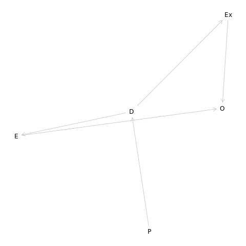
We should note that it seems straightforward, but it is nice to check as well.
1dag5m5 %>% adjustmentSets(exposure="P",outcome="O") %>% print
1
2 {}
Now we can start working our way through the set of regressions by the most basic walk through the DAG.
Path One
- \(D(P)\) decreases
- \(E_{x}(D)\) increases
- \(O(E_{x})\) decreases
Path Two
- \(D(P)\) decreases
- \(E(D)\) decreases
- \(O(E)\) decreases
Chapter VI: The Haunted DAG & The Causal Terror
Easy Questions (Ch6)
6E1
List three mechanisms by which multiple regression can produce false inferences about causal effects.
Solution
As per chapter five and six, we have three mechanisms:
- Confounding
- Where there exists an additional variable which influences exposure and outcome values
- Multicollinearity
- Strong associations between two or more predictor variables, which will cause the posterior distribution to suggest that none of variables are associated with the outcome even if they all actually are
- Post-treatment variables
- This is a form of included variable bias
- Collider Bias
- Conditioning on collider variables creates statistical but not causal associations between its causes
HOLD 6E2
For one of the mechanisms in the previous problem, provide an example of your choice, perhaps from your own research.
Solution
One of the core tenets of the field of computational chemistry is the act of fitting empirical potential models to more accurate potential data (or even experiments).
- Multicollinearity
- When dealing with decreasing effects, then using strongly correlated variables (like distance and effective distance measures like centeroid densities) cause the overall model to suggest that none of the measures are useful
- Post-treatment variables
- Often while finding minima and saddle points on a potential energy surface, adding information of the existing minima values will impede training a model which actually fits to the whole potential energy surface instead of being concentrated around the known minima
6E3
List the four elemental confounds. Can you explain the conditional dependencies of each?
Solution
The four elemental confounds are enumerated in Figure 1.
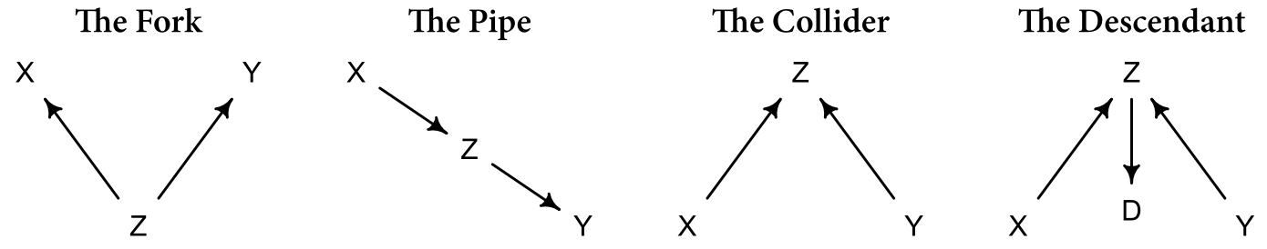
Figure 1: The four elemental confounds
In symbolic notation, we can express this as:
| Confound | Symbolic Form | Conditional Independencies |
|---|---|---|
| Forks | \(X←Z→Y\) | \(Y⫫ X\vert Z\) |
| Pipes | \(X → Z → Y\) | \(Y⫫ X\vert Z\) |
| Colliders | \(X→Z←Y\) | \(Y \not⫫ X\vert Z\) |
| Descendants | See Figure 1 | Weakly conditions on parent |
6E4
How is a biased sample like conditioning on a collider? Think of the example at the open of the chapter.
Solution
Recall that the biased sample in the introduction to the chapter was:
It seems like the most newsworthy scientific studies are the least trustworthy. The more likely it is to kill you, if true, the less likely it is to be true. The more boring the topic, the more rigorous the results. How could this widely believed negative correlation exist? There doesn’t seem to be any reason for studies of topics that people care about to produce less reliable results. Maybe popular topics attract more and worse researchers, like flies drawn to the smell of honey?
Note that this can also be expressed as a collider in a causal DAG as:
\[\mathrm{newsworthiness}→\mathrm{acceptance}←\mathrm{trustworthiness}\]
The idea is that a proposal will be accepted if either the newsworthiness or the trustworthiness is high. There is thus on average a negative association between these criteria among the selected set of proposals.
In essence the association in the sub-samples is not the same as the total sample, and this causes wrong inferences on the total sample set, when conditioning on collider variables.
Questions of Medium Complexity (Ch6)
6M1
Modify the DAG on page \(186\) to include the variable \(V\), an unobserved cause of \(C\) and \(Y:C\gets V \to Y\). Reanalyze the DAG. How many paths connect \(X\) to \(Y\)? Which must be closed? Which variables should you condition on now?
Solution
Let us outline this DAG.
 1dag6m1<- dagitty("dag{
 2U [unobserved]
 3V [unobserved]
 4X -> Y
 5X <- U -> B <- C -> Y
 6U <- A -> C
 7C <- V -> Y
 8}")
 9coordinates(dag6m1)<-list(
10  x=c(X=0,Y=2,U=0,A=1,B=1,C=2,V=2.5),
11  y=c(X=2,Y=2,U=1,A=0.2,B=1.5,C=1,V=1.5)
12)
We can visualize this with:
1dag6m1 %>% drawdag

The paths between \(X\) and \(Y\) are:
- \(X→Y\)
- \(X←U→A←C→Y\)
- \(X←U→A←C←V→Y\)
- \(X←U→B←C→Y\)
- \(X←U→B←C←V→Y\)
We can leverage dagitty to check which paths should be closed.
1dag6m1 %>% adjustmentSets(exposure="X",outcome="Y") %>% print
1 { A }
Logically, conditioning on \(A\) to close non-causal paths makes sense as it consistent with the understanding that only (1) is a causal path, and the rest will confound paths.
6M2
Sometimes in order to avoid multicollinearity, people inspect pairwise correlations among predictors before including them in a model. This is a bad procedure, because what matters is the conditional association, not the association before the variables are included in the model. To highlight this, consider the DAG \(X\to Z\to Y\). Simulate data from this DAG so that the correlation between \(X\) and \(Z\) is very large. Then include both in a model prediction \(Y\). Do you observe any multicollinearity? Why or why not? What is different from the legs example in the chapter?
Solution
The DAG under consideration is: \[ X\to Z\to Y \] We will simulate data first.
1N<-5000
2X<-N %>% rnorm(mean=0,sd=1)
3Z<-N %>% rnorm(mean=X,sd=0.5)
4Y<-N %>% rnorm(mean=Z,sd=1)
5cor(X,Z) %>% print
1
2[1] 0.9987166
The variables \(X\) and \(Z\) are highly correlated. We can check with a regression model for this.
1m6m2<-quap(
2  alist(
3    Y ~ dnorm(mu,sigma),
4    mu<-a+bX*X+bZ*Z,
5    c(a,bX,bZ)~dnorm(0,1),
6    sigma~dexp(1)
7  ), data=list(X=X,Y=Y,Z=Z)
8)
The regression fit is essentially.
1m6m2 %>% precis
1       mean   sd  5.5% 94.5%
2a     -0.01 0.01 -0.03  0.01
3bX     0.06 0.03  0.00  0.11
4bZ     0.95 0.03  0.90  1.00
5sigma  1.02 0.01  1.00  1.04
The fit shows how \(X\) is not a useful variable, due to the addition of \(Z\), which is a post-treatment variable, and thus should not have been included. In effect, we also realize from this that multicollinearity is a data-driven property, and has no interpretation outside specific model instances.
6M3
Learning to analyze DAGs requires practice. For each of the four DAGs below, state which variables, if any, you must adjust for (condition on) to estimate the total causal influence of \(X\) on \(Y\).
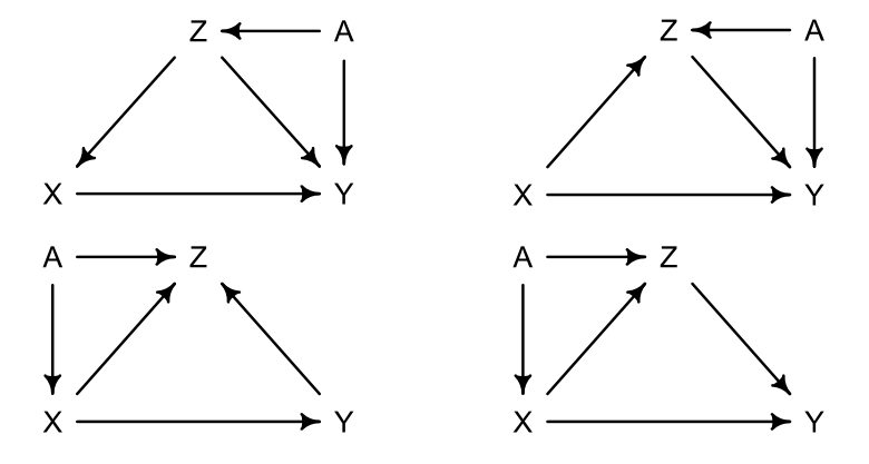
Solution
We can leverage the dagitty package as well to figure out which variables should be conditioned on.
 1dag6m3a<- dagitty("dag{
 2X -> Y
 3X <- Z -> Y
 4X <- Z <- A -> Y
 5}")
 6dag6m3b<- dagitty("dag{
 7X -> Y
 8X -> Z -> Y
 9X -> Z <- A -> Y
10}")
11dag6m3c<- dagitty("dag{
12X -> Y
13X -> Z <- Y
14X <- A -> Z <- Y
15}")
16dag6m3d<- dagitty("dag{
17X -> Y
18X -> Z -> Y
19X <- A -> Z -> Y
20}")
1dag6m3a %>% adjustmentSets(exposure="X",outcome="Y") %>% print
2dag6m3b %>% adjustmentSets(exposure="X",outcome="Y") %>% print
3dag6m3c %>% adjustmentSets(exposure="X",outcome="Y") %>% print
4dag6m3d %>% adjustmentSets(exposure="X",outcome="Y") %>% print
1 { Z }
2
3 {}
4
5 {}
6
7 { A }
Clearly the upper left and lower right DAGs need to be conditioned on Z and A respectively to close non-causal paths.
We can further rationalize this as follows:
- Upper Left
- \(X\gets Z\to Y\) and \(X\gets Z \gets A \to Y\) are open, non-causal paths which need to be closed
- Upper Right
- \(Z\) is a collider which ensures that only causal paths are open
- Lower Left
- There is a collider \(Z\) which ensures that the non-causal paths are closed
- Lower Right
- This figure is more complicated, so we will consider all the paths, i.e. \(X \to Y\), \(X \to Z \to Y\), \(X\gets A \to Z\to Y\), and we clearly need to condition on either \(A\) or \(Z\). \(Z\) is also part of a causal path, so only \(A\) is to be conditioned on
A more canonical way to do this is to enumerate all paths for every option, but dagitty is more elegant.
1dag6m3d %>% graphLayout %>% plot
Chapter VII: Ulysses’ Compass
Easy Questions (Ch7)
HOLD 7E1
State the three motivating criteria that define information entropy. Try to express each in your own words.
Solution
The motivating criteria for defining informational entropy or “uncertainity” are:
- Continuity
- It is preferable to have a continuous function to define our informational criteria, since we can always discretize a continuous function (by binning) later, but a discrete function does not have a full range of values which can correspond to all the possible models. As a metric then, it is preferable to have a minimum and maximum bound, but define it such that it is continuous for representing arbitrary models
- Positive and Monotonic
- The monotonicity constraint is simply to ensure that as the number of events increases, given no other changes in the system, the uncertainity will increase. Since the function is already continuous, the incerasing nature is really by construction. It should be noted that a monotonously decreasing function would also satisfy the motivating criteria, but will change the interpretation completely
- Additivity
- As mentioned for continuity, it is possible always to bin continuous functions or discretize it. Similarly, it is desirable to keep the amount of uncertainity constant and add or subtract values to redefine categories
7E2
Suppose a coin is weighted such that, when it is tossed and lands on a table, it comes up heads \(70\%\) of the time. What is the entropy of this coin?
Solution
We can simulate this system easily.
1p<-c(0.7,0.3)
2-sum(p*log(p)) %>% print
1[1] 0.6108643
7E3
Suppose a four-sided die is loaded such that, when tossed onto a table, it shows “1” \(20\%\), “2”, \(25\%\), and “4” \(30\%\) of the time. What is the entropy of this die?
Solution
1p<-c(0.2,0.25,0.25,0.3)
2-sum(p*log(p)) %>% print
1[1] 1.376227
7E4
Suppose another four-sided die is loaded such that it never shows “4”. The other three sides show equally often. What is the entropy of this die?
Solution
We will not consider impossible events in our simulation.
1p<- c(1/3,1/3,1/3)
2-sum(p*log(p)) %>% print
1[1] 1.098612
Questions of Medium Complexity (Ch7)
HOLD 7M1
Write down and compare the definitions of AIC and WAIC. Which of these criteria is most general? Which assumptions are required to transform the more general criterion into a less general one?
Solution
We know that AIC or “Akaike Information Criterion” is defined as:
Where \(k\) is the number of parameters in the model.
The WAIC or “Widely Applicable Information Criterion” is given by: \[\mathrm{WAIC}=-2\left(\sum_{i}\log\Pr(y_{i})-\sum_{i}V(y_{i})\right)\]
WAIC is more general than the AIC. WAIC and AIC will be approximately equivalent when the priors are effectively flat or when there is enough data to render the priors redundant. This is because the WAIC makes no assumptions about the shape of the posterior, while AIC is an approximation depending on:
- A flat prior (or one overwhelmed by the likelihood)
- A posterior distribution which is approximately a multivariate Gaussian
- Sample size \(N\) with more parameters (\(p\))
Furthermore, we note that the AIC simply estimates that the penalty term is twice the number of parameters, while the WAIC fits uses the lppd or the sum of variances of each log-likelihood.
HOLD 7M2
Explain the difference between model selection and model comparison. What information is lost under model selection?
Solution
Model selection involves choosing one model over the others. Ideally this occurs after appropriate model comparision. However, the chapter does mention that it is common to use heuristics like “stargazing” which uses frequentist tools to estimate which variables are important, then choose a model (or causal salad)a which has the highest number of significant variables.
Model comparision in theory should be based off entropic measures for the information used. The models should be trained on the same data-set for the metrics to be meaningful.
Model selection loses information regarding the uncertainity quantifications of the models which do not necessarily have the (relatively) optimal values of the metric used for comparision. This is important, especially since models which are parameterized for prediction, often perform better without being useful for causal analysis.
7M3
When comparing models with an information criterion, why must all models be fit to exactly the same observations? What would happen to the information criterion values, if the models were fit to different numbers of observations? Perform some experiments, if you are not sure.
Solution
When using an information criterion, it is important to understand that different values define different “small worlds”.
This is why when working on gauging the information criterion, which work on the basis of the accumulated deviance values, having a varying number of training values will effectively be comparing apples and oranges. Each training data-set essentially fits one model, and comparing models trained on different data-sets (even subsets of the same data) will not lead to a fundamentally sound comparison.
We also know that in general, fewer data-points will have fewer deviance terms, and therefore artificially seem to be better.
We will prove this with an artificial data-set.
 1ySmallDat <- rnorm(100)
 2yLargeDat <- rnorm(1000)
 3m7m3S <- quap(
 4  alist(
 5    y ~ dnorm(mu,1),
 6    mu ~ dnorm(0,sigma)
 7  ), data=list(y=ySmallDat,sigma=1)
 8)
 9m7m3L <- quap(
10  alist(
11    y ~ dnorm(mu,1),
12    mu ~ dnorm(0,sigma)
13  ),data=list(y=yLargeDat,sigma=1)
14)
1WAIC(m7m3S) %>% rbind(WAIC(m7m3L)) %>% mutate(numSamples=c(100,1000)) %>% toOrg
| WAIC | lppd | penalty | std_err | numSamples |
|---|---|---|---|---|
| 278.876677095335 | -138.576629006818 | 0.861709540849766 | 11.1055429875975 | 100 |
| 2898.5831283182 | -1448.20174278015 | 1.08982137894866 | 49.5298847525459 | 1000 |
We see that apparently, the model with fewer data-points is superior, but from the discussion above, as well as by construction, we know that the models are the same, so the effect is clearly spurious, and caused by training on different data-sets.
7M4
What happens to the effective number of parameters as measured by PSIS or WAIC, as a prior becomes more concentrated? Why? Perform some experiments, if you are not sure.
Solution
Since a strength of a prior is directly related to the process of regularization, it is clear that as a prior becomes more concentrated, the model tends to be more critical of new data, and therefore the effective number of parameters will drop proportionately. Another approach to the same problem is to understand that the prior encodes our previous beliefs which in effect represents additional data which the model a-priori has been trained with.
We can test this simply by re-using the models we defined for 7M3.
 1yDat <- rnorm(5)
 2sigL<-1000
 3sigS<-1
 4m7m4S <- quap(
 5  alist(
 6    y ~ dnorm(mu,1),
 7    mu ~ dnorm(0,sigma)
 8  ), data=list(y=yDat,sigma=sigS)
 9)
10m7m4L <- quap(
11  alist(
12    y ~ dnorm(mu,1),
13    mu ~ dnorm(0,sigma)
14  ),data=list(y=yDat,sigma=sigL)
15)
Recall that the WAIC is defined by:
\[ WAIC = -2(lppd-pWAIC) \]
Where pWAIC is the effective number of parameters. So we note that:
\[ pWAIC=lppd-0.5*WAIC \]
This is reported by WAIC as the penalty parameter.
1WAIC(m7m4S) %>% rbind(WAIC(m7m4L)) %>% mutate(sigma=c(sigS,sigL)) %>% toOrg
| WAIC | lppd | penalty | std_err | sigma |
|---|---|---|---|---|
| 16.4098404638955 | -7.31440324407321 | 0.890516987874561 | 2.31086161575483 | 1 |
| 16.9915093637752 | -7.3011838990595 | 1.19457078282808 | 2.5268591022024 | 1000 |
Though the effect is not too strong, it is clear that having a denser prior (a.k.a smaller sigma) has a smaller number of effective paramters, as expected.
HOLD 7M5
Provide an informal explanation of why informative priors reduce overfitting.
Solution
Overfitting is easier to understand in the context of data-compression. Essentially, when overfitting occurs, the data is represented in a different encoding, instead of being compressed.
We can also look at the overfitting process to be a trade off between simply fitting to every data-point (low bias, high variance) and being completely oblivious to the data (high bias, low variance). In another sense, overfitting occurs when the model is “overly eager” to learn from the data.
Given this understanding, informative priors essentially regularize the model, by ensuring that the likelihood is closer to the posterior, and hence prevents the model from “learning” from data-points which are not actually relevant to the prior.
This implies that overfitting reduces the model by lowering the sensitivity of the model to a sample, which implicitly implies that the data contains points which are not actually a feature of the process which will generate future data.
HOLD 7M6
Provide an informal explanation of why overly informative priors result in underfitting.
Solution
Underfitting occurs when the model is insensitive to newer samples of the data. In classical terms, this means that the model has a very high bias, and typically has a correspondingly low variance.
With the understanding that priors cause regularization, which enforces sparsity of features, it is easier to see that very strong priors ensure that the model is overly sparse and incapable of picking up relevant trends in the training data.
Overly informative priors, essentially imply that the model has “seen” a large amount of data previously, which then means that it is less sensitive to newer samples of data. This means that features present in the training data which are relevant to future data will be ignored in favor of the prior predictions.
A: Colophon
To ensure that this document is fully reproducible at a later date, we will record the session info.
1devtools::session_info()
  1- Session info ---------------------------------------------------------------
  2 setting  value
  3 version  R version 4.0.0 (2020-04-24)
  4 os       Arch Linux
  5 system   x86_64, linux-gnu
  6 ui       X11
  7 language (EN)
  8 collate  C
  9 ctype    C
 10 tz       Iceland
 11 date     2020-06-13
 12
 13- Packages -------------------------------------------------------------------
 14 package              * version    date       lib   source
 15 arrayhelpers           1.1-0      2020-02-04 [167] CRAN (R 4.0.0)
 16 assertthat             0.2.1      2019-03-21 [34]  CRAN (R 4.0.0)
 17 backports              1.1.6      2020-04-05 [68]  CRAN (R 4.0.0)
 18 boot                   1.3-24     2019-12-20 [5]   CRAN (R 4.0.0)
 19 broom                  0.5.6      2020-04-20 [67]  CRAN (R 4.0.0)
 20 callr                  3.4.3      2020-03-28 [87]  CRAN (R 4.0.0)
 21 cellranger             1.1.0      2016-07-27 [55]  CRAN (R 4.0.0)
 22 cli                    2.0.2      2020-02-28 [33]  CRAN (R 4.0.0)
 23 coda                   0.19-3     2019-07-05 [169] CRAN (R 4.0.0)
 24 colorspace             1.4-1      2019-03-18 [97]  CRAN (R 4.0.0)
 25 crayon                 1.3.4      2017-09-16 [35]  CRAN (R 4.0.0)
 26 curl                   4.3        2019-12-02 [26]  CRAN (R 4.0.0)
 27 dagitty              * 0.2-2      2016-08-26 [244] CRAN (R 4.0.0)
 28 data.table           * 1.12.8     2019-12-09 [27]  CRAN (R 4.0.0)
 29 DBI                    1.1.0      2019-12-15 [77]  CRAN (R 4.0.0)
 30 dbplyr                 1.4.3      2020-04-19 [76]  CRAN (R 4.0.0)
 31 desc                   1.2.0      2018-05-01 [84]  CRAN (R 4.0.0)
 32 devtools             * 2.3.0      2020-04-10 [219] CRAN (R 4.0.0)
 33 digest                 0.6.25     2020-02-23 [42]  CRAN (R 4.0.0)
 34 dplyr                * 0.8.5      2020-03-07 [69]  CRAN (R 4.0.0)
 35 ellipsis               0.3.0      2019-09-20 [30]  CRAN (R 4.0.0)
 36 evaluate               0.14       2019-05-28 [82]  CRAN (R 4.0.0)
 37 fansi                  0.4.1      2020-01-08 [36]  CRAN (R 4.0.0)
 38 forcats              * 0.5.0      2020-03-01 [29]  CRAN (R 4.0.0)
 39 fs                     1.4.1      2020-04-04 [109] CRAN (R 4.0.0)
 40 generics               0.0.2      2018-11-29 [71]  CRAN (R 4.0.0)
 41 ggplot2              * 3.3.0      2020-03-05 [78]  CRAN (R 4.0.0)
 42 glue                 * 1.4.0      2020-04-03 [37]  CRAN (R 4.0.0)
 43 gridExtra              2.3        2017-09-09 [123] CRAN (R 4.0.0)
 44 gtable                 0.3.0      2019-03-25 [79]  CRAN (R 4.0.0)
 45 haven                  2.2.0      2019-11-08 [28]  CRAN (R 4.0.0)
 46 hms                    0.5.3      2020-01-08 [44]  CRAN (R 4.0.0)
 47 htmltools              0.4.0      2019-10-04 [112] CRAN (R 4.0.0)
 48 httr                   1.4.1      2019-08-05 [100] CRAN (R 4.0.0)
 49 inline                 0.3.15     2018-05-18 [162] CRAN (R 4.0.0)
 50 jsonlite               1.6.1      2020-02-02 [101] CRAN (R 4.0.0)
 51 kableExtra           * 1.1.0      2019-03-16 [212] CRAN (R 4.0.0)
 52 knitr                  1.28       2020-02-06 [113] CRAN (R 4.0.0)
 53 latex2exp            * 0.4.0      2015-11-30 [211] CRAN (R 4.0.0)
 54 lattice                0.20-41    2020-04-02 [6]   CRAN (R 4.0.0)
 55 lifecycle              0.2.0      2020-03-06 [38]  CRAN (R 4.0.0)
 56 loo                    2.2.0      2019-12-19 [163] CRAN (R 4.0.0)
 57 lubridate              1.7.8      2020-04-06 [106] CRAN (R 4.0.0)
 58 magrittr               1.5        2014-11-22 [21]  CRAN (R 4.0.0)
 59 MASS                   7.3-51.5   2019-12-20 [7]   CRAN (R 4.0.0)
 60 matrixStats            0.56.0     2020-03-13 [164] CRAN (R 4.0.0)
 61 memoise                1.1.0      2017-04-21 [229] CRAN (R 4.0.0)
 62 modelr                 0.1.6      2020-02-22 [107] CRAN (R 4.0.0)
 63 munsell                0.5.0      2018-06-12 [96]  CRAN (R 4.0.0)
 64 mvtnorm                1.1-0      2020-02-24 [243] CRAN (R 4.0.0)
 65 nlme                   3.1-147    2020-04-13 [11]  CRAN (R 4.0.0)
 66 orgutils             * 0.4-1      2017-03-21 [209] CRAN (R 4.0.0)
 67 pillar                 1.4.3      2019-12-20 [39]  CRAN (R 4.0.0)
 68 pkgbuild               1.0.6      2019-10-09 [86]  CRAN (R 4.0.0)
 69 pkgconfig              2.0.3      2019-09-22 [43]  CRAN (R 4.0.0)
 70 pkgload                1.0.2      2018-10-29 [83]  CRAN (R 4.0.0)
 71 plyr                   1.8.6      2020-03-03 [73]  CRAN (R 4.0.0)
 72 prettyunits            1.1.1      2020-01-24 [58]  CRAN (R 4.0.0)
 73 printr               * 0.1        2017-05-19 [214] CRAN (R 4.0.0)
 74 processx               3.4.2      2020-02-09 [88]  CRAN (R 4.0.0)
 75 ps                     1.3.2      2020-02-13 [89]  CRAN (R 4.0.0)
 76 purrr                * 0.3.4      2020-04-17 [50]  CRAN (R 4.0.0)
 77 R6                     2.4.1      2019-11-12 [48]  CRAN (R 4.0.0)
 78 Rcpp                   1.0.4.6    2020-04-09 [10]  CRAN (R 4.0.0)
 79 readr                * 1.3.1      2018-12-21 [45]  CRAN (R 4.0.0)
 80 readxl                 1.3.1      2019-03-13 [54]  CRAN (R 4.0.0)
 81 remotes                2.1.1      2020-02-15 [233] CRAN (R 4.0.0)
 82 reprex                 0.3.0      2019-05-16 [108] CRAN (R 4.0.0)
 83 rethinking           * 2.01       2020-06-06 [242] local
 84 rlang                  0.4.5      2020-03-01 [31]  CRAN (R 4.0.0)
 85 rmarkdown              2.1        2020-01-20 [110] CRAN (R 4.0.0)
 86 rprojroot              1.3-2      2018-01-03 [85]  CRAN (R 4.0.0)
 87 rstan                * 2.19.3     2020-02-11 [161] CRAN (R 4.0.0)
 88 rstudioapi             0.11       2020-02-07 [91]  CRAN (R 4.0.0)
 89 rvest                  0.3.5      2019-11-08 [120] CRAN (R 4.0.0)
 90 scales                 1.1.0      2019-11-18 [93]  CRAN (R 4.0.0)
 91 sessioninfo            1.1.1      2018-11-05 [231] CRAN (R 4.0.0)
 92 shape                  1.4.4      2018-02-07 [193] CRAN (R 4.0.0)
 93 StanHeaders          * 2.19.2     2020-02-11 [165] CRAN (R 4.0.0)
 94 stringi                1.4.6      2020-02-17 [52]  CRAN (R 4.0.0)
 95 stringr              * 1.4.0      2019-02-10 [74]  CRAN (R 4.0.0)
 96 svUnit                 1.0.3      2020-04-20 [168] CRAN (R 4.0.0)
 97 testthat               2.3.2      2020-03-02 [81]  CRAN (R 4.0.0)
 98 textutils              0.2-0      2020-01-07 [210] CRAN (R 4.0.0)
 99 tibble               * 3.0.1      2020-04-20 [32]  CRAN (R 4.0.0)
100 tidybayes            * 2.0.3      2020-04-04 [166] CRAN (R 4.0.0)
101 tidybayes.rethinking * 2.0.3.9000 2020-06-07 [246] local
102 tidyr                * 1.0.2      2020-01-24 [75]  CRAN (R 4.0.0)
103 tidyselect             1.0.0      2020-01-27 [49]  CRAN (R 4.0.0)
104 tidyverse            * 1.3.0      2019-11-21 [66]  CRAN (R 4.0.0)
105 usethis              * 1.6.0      2020-04-09 [238] CRAN (R 4.0.0)
106 V8                     3.0.2      2020-03-14 [245] CRAN (R 4.0.0)
107 vctrs                  0.2.4      2020-03-10 [41]  CRAN (R 4.0.0)
108 viridisLite            0.3.0      2018-02-01 [99]  CRAN (R 4.0.0)
109 webshot                0.5.2      2019-11-22 [213] CRAN (R 4.0.0)
110 withr                  2.2.0      2020-04-20 [90]  CRAN (R 4.0.0)
111 xfun                   0.13       2020-04-13 [116] CRAN (R 4.0.0)
112 xml2                   1.3.2      2020-04-23 [122] CRAN (R 4.0.0)
113
114[1] /nix/store/xzd8h53xkyvfm3kvj5ab6znp685wi04w-r-car-3.0-7/library
115[2] /nix/store/mhr8zw9bmxarc3n821b83i0gz2j9zlrq-r-abind-1.4-5/library
116[3] /nix/store/hp86nhr0787vib3l8mkw0gf9nxwb45im-r-carData-3.0-3/library
117[4] /nix/store/vhw7s2h5ds6sp110z2yvilchv8j9jch5-r-lme4-1.1-23/library
118[5] /nix/store/987n8g0zy9sjvfvnsck1bkkcknw05yvb-r-boot-1.3-24/library
119[6] /nix/store/jxxxxyz4c1k5g3drd35gsrbjdg028d11-r-lattice-0.20-41/library
120[7] /nix/store/q9zfm5h53m8rd08xcsdcwaag31k4z1pf-r-MASS-7.3-51.5/library
121[8] /nix/store/kjkm50sr144yvrhl5axfgykbiy13pbmg-r-Matrix-1.2-18/library
122[9] /nix/store/8786z5lgy8h3akfjgj3yq5yq4s17rhjy-r-minqa-1.2.4/library
123[10] /nix/store/93wv3j0z1nzqp6fjsm9v7v8bf8d1xkm2-r-Rcpp-1.0.4.6/library
124[11] /nix/store/akfw6zsmawmz8lmjkww0rnqrazm4mqp0-r-nlme-3.1-147/library
125[12] /nix/store/rxs0d9bbn8qhw7wmkfb21yk5abp6lpq1-r-nloptr-1.2.2.1/library
126[13] /nix/store/8n0jfiqn4275i58qgld0dv8zdaihdzrk-r-RcppEigen-0.3.3.7.0/library
127[14] /nix/store/8vxrma33rhc96260zsi1jiw7dy3v2mm4-r-statmod-1.4.34/library
128[15] /nix/store/2y46pb5x9lh8m0hdmzajnx7sc1bk9ihl-r-maptools-0.9-9/library
129[16] /nix/store/iwf9nxx1v883wlv0p88q947hpz5lhfh7-r-foreign-0.8-78/library
130[17] /nix/store/rl9sjqply6rjbnz5k792ghm62ybv76px-r-sp-1.4-1/library
131[18] /nix/store/ws4bkzyv2vj5pyn1hgwyy6nlp48arz0n-r-mgcv-1.8-31/library
132[19] /nix/store/307dzxrmnqk4p86560a02r64x1fhhmxb-r-nnet-7.3-13/library
133[20] /nix/store/g2zpzkdb9hzkza1wpcbrk58119v1wyaf-r-pbkrtest-0.4-8.6/library
134[21] /nix/store/p0l503fr8960vld70w6ilmknxs5qwq77-r-magrittr-1.5/library
135[22] /nix/store/rmjpcaw3i446kwnjgcxcaid0yac36cj2-r-quantreg-5.55/library
136[23] /nix/store/10mzmnvc5jjgk2xzasia522pk60a30qz-r-MatrixModels-0.4-1/library
137[24] /nix/store/6qwdzvmnnmhjwdnvg2zmvv6wafd1vf91-r-SparseM-1.78/library
138[25] /nix/store/aa9c39a3yiqkh1h7pbngjlbr7czvc7yi-r-rio-0.5.16/library
139[26] /nix/store/2fx4vqlybgwp5rhhy6pssqx7h1a927fn-r-curl-4.3/library
140[27] /nix/store/k4m3fn1kqvvvn8y33kd57gq49hr3ar8y-r-data.table-1.12.8/library
141[28] /nix/store/651hfjylqzmsf565wyx474vyjny771gy-r-haven-2.2.0/library
142[29] /nix/store/a3rnz28irmqvmj8axj5x5j1am2c3gzs4-r-forcats-0.5.0/library
143[30] /nix/store/j8v4gzib137q2cml31hvvfkrc0f60pp5-r-ellipsis-0.3.0/library
144[31] /nix/store/xaswqlnamf4k8vwx0x3wav3l0x60sag0-r-rlang-0.4.5/library
145[32] /nix/store/dqm3xpix2jwhhhr67s6fgrwbw7hizap7-r-tibble-3.0.1/library
146[33] /nix/store/v7xfsq6d97wpn6m0hjrac78w5xawbr8a-r-cli-2.0.2/library
147[34] /nix/store/fikjasr98klhk9cf44x4lhi57vh3pmkg-r-assertthat-0.2.1/library
148[35] /nix/store/3fya6cd38vsqdj0gjb7bcsy00sirlyw1-r-crayon-1.3.4/library
149[36] /nix/store/payqi9bwh216rwhaq07jgc26l4fv1zsb-r-fansi-0.4.1/library
150[37] /nix/store/h6a61ghws7yrdxlg412xl1im37z5r28i-r-glue-1.4.0/library
151[38] /nix/store/y8mjbia1wbnq26dkigr0p3xxwrbzsc2r-r-lifecycle-0.2.0/library
152[39] /nix/store/kwaghh12cnifgvcbvlv2anx0hd5f4ild-r-pillar-1.4.3/library
153[40] /nix/store/k1phn8j10nni7gzvcgp0vc25dby6bb77-r-utf8-1.1.4/library
154[41] /nix/store/k3b77y8v7zsshpp1ccs8jwk2i2g4rm9a-r-vctrs-0.2.4/library
155[42] /nix/store/iibjmbh7vj0d0bfafz98yn29ymg43gkw-r-digest-0.6.25/library
156[43] /nix/store/aqsj4k3pgm80qk4jjg7sh3ac28n6alv0-r-pkgconfig-2.0.3/library
157[44] /nix/store/i7c5v8s4hd9rlqah3bbvy06yywjqwdgk-r-hms-0.5.3/library
158[45] /nix/store/2fyrk58cmcbrxid66rbwjli7y114lvrm-r-readr-1.3.1/library
159[46] /nix/store/163xq2g5nblqgh7qhvzb6mvgg6qdrirj-r-BH-1.72.0-3/library
160[47] /nix/store/dr27b6k49prwgrjs0v30b6mf5lxa36pk-r-clipr-0.7.0/library
161[48] /nix/store/bghvqg9mcaj2jkbwpy0di6c563v24acz-r-R6-2.4.1/library
162[49] /nix/store/nq8jdq7nlg9xns4xpgyj6sqv8p4ny1wz-r-tidyselect-1.0.0/library
163[50] /nix/store/zlwhf75qld7vmwx3d4bdws057ld4mqbp-r-purrr-0.3.4/library
164[51] /nix/store/0gbmmnbpqlr69l573ymkcx8154fvlaca-r-openxlsx-4.1.4/library
165[52] /nix/store/1m1q4rmwx56dvx9rdzfsfq0jpw3hw0yx-r-stringi-1.4.6/library
166[53] /nix/store/mhy5vnvbsl4q7dcinwx3vqlyywxphbfd-r-zip-2.0.4/library
167[54] /nix/store/88sp7f7q577i6l5jjanqiv5ak6nv5357-r-readxl-1.3.1/library
168[55] /nix/store/6q9zwivzalhmzdracc8ma932wirq8rl5-r-cellranger-1.1.0/library
169[56] /nix/store/jh2n6k2ancdzqych5ix8n4rq9w514qq9-r-rematch-1.0.1/library
170[57] /nix/store/22xjqikqd6q556absb5224sbx6q0kp0c-r-progress-1.2.2/library
171[58] /nix/store/9vp32wa1qvv6lkq6p70qlli5whrxzfbi-r-prettyunits-1.1.1/library
172[59] /nix/store/r9rhqb6fsk75shihmb7nagqb51pqwp0y-r-class-7.3-16/library
173[60] /nix/store/z1kad071y43wij1ml9lpghh7jbimmcli-r-cluster-2.1.0/library
174[61] /nix/store/i8wr965caf6j1rxs2dsvpzhlh4hyyb4y-r-codetools-0.2-16/library
175[62] /nix/store/8iglq3zr68a39hzswvzxqi2ffhpw9p51-r-KernSmooth-2.23-16/library
176[63] /nix/store/n3k50zv40i40drpdf8npbmy2y08gkr6w-r-rpart-4.1-15/library
177[64] /nix/store/b4r6adzcvpm8ivflsmis7ja7q4r5hkjy-r-spatial-7.3-11/library
178[65] /nix/store/zqg6hmrncl8ax3vn7z5drf4csddwnhcx-r-survival-3.1-12/library
179[66] /nix/store/4anrihkx11h8mzb269xdyi84yp5v7grl-r-tidyverse-1.3.0/library
180[67] /nix/store/945haq0w8nfm9ib7r0nfngn5lk2i15ix-r-broom-0.5.6/library
181[68] /nix/store/52viqxzrmxl7dk0zji293g5b0b9grwh8-r-backports-1.1.6/library
182[69] /nix/store/zp1k42sw2glqy51w4hnzsjs8rgi8xzx2-r-dplyr-0.8.5/library
183[70] /nix/store/mkjd98mnshch2pwnj6h31czclqdaph3f-r-plogr-0.2.0/library
184[71] /nix/store/kflrzax6y5pwfqwzgfvqz433a3q3hnhn-r-generics-0.0.2/library
185[72] /nix/store/xi1n5h5w17c33y6ax3dfhg2hgzjl9bxz-r-reshape2-1.4.4/library
186[73] /nix/store/vn63z92zkpbaxmmhzpb6mq2fvg0xa26h-r-plyr-1.8.6/library
187[74] /nix/store/wmpyxss67bj44rin7hlnr9qabx66p5hj-r-stringr-1.4.0/library
188[75] /nix/store/330qbgbvllwz3h0i2qidrlk50y0mbgph-r-tidyr-1.0.2/library
189[76] /nix/store/cx3x4pqb65l1mhss65780hbzv9jdrzl6-r-dbplyr-1.4.3/library
190[77] /nix/store/gsj49bp3hpw9jlli3894c49amddryqsq-r-DBI-1.1.0/library
191[78] /nix/store/kvymhwp4gac0343c2yi1qvdpavx4gdn2-r-ggplot2-3.3.0/library
192[79] /nix/store/knv51jvpairvibrkkq48b6f1l2pa1cv8-r-gtable-0.3.0/library
193[80] /nix/store/158dx0ddv20ikwag2860nlg9p3hbh1zc-r-isoband-0.2.1/library
194[81] /nix/store/fprs9rp1jlhxzj7fp6l79akyf8k3p7zd-r-testthat-2.3.2/library
195[82] /nix/store/0pmlnkyn0ir3k9bvxihi1r06jyl64w3i-r-evaluate-0.14/library
196[83] /nix/store/7210bjjqn5cjndxn5isnd4vip00xhkhy-r-pkgload-1.0.2/library
197[84] /nix/store/9a12ybd74b7dns40gcfs061wv7913qjy-r-desc-1.2.0/library
198[85] /nix/store/na9pb1apa787zp7vvyz1kzym0ywjwbj0-r-rprojroot-1.3-2/library
199[86] /nix/store/pa2n7bh61qxyarn5i2ynd62k6knb1np1-r-pkgbuild-1.0.6/library
200[87] /nix/store/1hxm1m7h4272zxk9bpsaq46mvnl0dbss-r-callr-3.4.3/library
201[88] /nix/store/bigvyk6ipglbiil93zkf442nv4y3xa1x-r-processx-3.4.2/library
202[89] /nix/store/370lr0wf7qlq0m72xnmasg2iahkp2n52-r-ps-1.3.2/library
203[90] /nix/store/rr72q61d8mkd42zc5fhcd2rqjghvc141-r-withr-2.2.0/library
204[91] /nix/store/9gw77p7fmz89fa8wi1d9rvril6hd4sxy-r-rstudioapi-0.11/library
205[92] /nix/store/9x4v4pbrgmykbz2801h77yz2l0nmm5nb-r-praise-1.0.0/library
206[93] /nix/store/pf8ssb0dliw5bzsncl227agc8przb7ic-r-scales-1.1.0/library
207[94] /nix/store/095z4wgjrxn63ixvyzrj1fm1rdv6ci95-r-farver-2.0.3/library
208[95] /nix/store/5aczj4s7i9prf5i32ik5ac5baqvjwdb1-r-labeling-0.3/library
209[96] /nix/store/wch26phipzz9gxd4vbr4fynh7v28349j-r-munsell-0.5.0/library
210[97] /nix/store/3w8fh756mszhsjx5fwgwydcpn8vkwady-r-colorspace-1.4-1/library
211[98] /nix/store/8cmaj81v2vm4f8p59ylbnsby8adkbmhd-r-RColorBrewer-1.1-2/library
212[99] /nix/store/h4x4ygax7gpz6f0c2v0xacr62080qwb8-r-viridisLite-0.3.0/library
213[100] /nix/store/qhx0i2nn5syb6vygdn8fdxgl7k56yj81-r-httr-1.4.1/library
214[101] /nix/store/lxnb4aniv02i4jhdvz02aaql1kznbpxb-r-jsonlite-1.6.1/library
215[102] /nix/store/13dcry4gad3vfwqzqb0ii4n06ybrxybr-r-mime-0.9/library
216[103] /nix/store/2can5l8gscc92a3bqlak8hfcg96v5hvf-r-openssl-1.4.1/library
217[104] /nix/store/piwsgxdz5w2ak8c6fcq0lc978qbxwdp1-r-askpass-1.1/library
218[105] /nix/store/3sj5h6dwa1l27d2hvdchclygk0pgffsr-r-sys-3.3/library
219[106] /nix/store/2z0p88g0c03gigl2ip60dlsfkdv1k30h-r-lubridate-1.7.8/library
220[107] /nix/store/1pkmj8nqjg2iinrkg2w0zkwq0ldc01za-r-modelr-0.1.6/library
221[108] /nix/store/bswkzvn8lczwbyw3y7n0p0qp2q472s0g-r-reprex-0.3.0/library
222[109] /nix/store/yid22gad8z49q52d225vfba2m4cgj2lx-r-fs-1.4.1/library
223[110] /nix/store/d185qiqaplm5br9fk1pf29y0srlabw83-r-rmarkdown-2.1/library
224[111] /nix/store/iszqviydsdj31c3ww095ndqy1ld3cibs-r-base64enc-0.1-3/library
225[112] /nix/store/i89wfw4cr0fz3wbd7cg44fk4dwz8b6h1-r-htmltools-0.4.0/library
226[113] /nix/store/qrl28laqwmhpwg3dpcf4nca8alv0px0g-r-knitr-1.28/library
227[114] /nix/store/jffaxc4a3bbf2g6ip0gdcya73dmg53mb-r-highr-0.8/library
228[115] /nix/store/717srph13qpnbzmgsvhx25q8pl51ivpj-r-markdown-1.1/library
229[116] /nix/store/mxqmyq3ybdfyc6p0anhfy2kfw0iz5k4n-r-xfun-0.13/library
230[117] /nix/store/b8g6hadva0359l6j1aq4dbvxlqf1acxc-r-yaml-2.2.1/library
231[118] /nix/store/rrl05vpv7cw58zi0k9ykm7m4rjb9gjv3-r-tinytex-0.22/library
232[119] /nix/store/2ziq8nzah6xy3dgmxgim9h2wszz1f89f-r-whisker-0.4/library
233[120] /nix/store/540wbw4p1g2qmnmbfk0rhvwvfnf657sj-r-rvest-0.3.5/library
234[121] /nix/store/n3prn77gd9sf3z4whqp86kghr55bf5w8-r-selectr-0.4-2/library
235[122] /nix/store/gv28yjk5isnglq087y7767xw64qa40cw-r-xml2-1.3.2/library
236[123] /nix/store/693czdcvkp6glyir0mi8cqvdc643whvc-r-gridExtra-2.3/library
237[124] /nix/store/3sykinp7lyy70dgzr0fxjb195nw864dv-r-future-1.17.0/library
238[125] /nix/store/bqi2l53jfxncks6diy0hr34bw8f86rvk-r-globals-0.12.5/library
239[126] /nix/store/dydyl209klklzh69w9q89f2dym9xycnp-r-listenv-0.8.0/library
240[127] /nix/store/lni0bi36r4swldkx7g4hql7gfz9b121b-r-gganimate-1.0.5/library
241[128] /nix/store/hh92jxs79kx7vxrxr6j6vin1icscl4k7-r-tweenr-1.0.1/library
242[129] /nix/store/0npx3srjnqgh7bib80xscjqvfyzjvimq-r-GGally-1.5.0/library
243[130] /nix/store/x5nzxklmacj6l162g7kg6ln9p25r3f17-r-reshape-0.8.8/library
244[131] /nix/store/q29z7ckdyhfmg1zlzrrg1nrm36ax756j-r-ggfortify-0.4.9/library
245[132] /nix/store/1rvm1w9iv2c5n22p4drbjq8lr9wa2q2r-r-cowplot-1.0.0/library
246[133] /nix/store/rp8jhnasaw1vbv5ny5zx0mw30zgcp796-r-ggrepel-0.8.2/library
247[134] /nix/store/wb7y931mm8nsj7w9xin83bvbaq8wvi4d-r-corrplot-0.84/library
248[135] /nix/store/gdzcqivfvgdrsz247v5kmnnw1v6p9c1p-r-rpart.plot-3.0.8/library
249[136] /nix/store/6yqg37108r0v22476cm2kv0536wyilki-r-caret-6.0-86/library
250[137] /nix/store/6fjdgcwgisiqz451sg5fszxnn9z8vxg6-r-foreach-1.5.0/library
251[138] /nix/store/c3ph5i341gk7jdinrkkqf6y631xli424-r-iterators-1.0.12/library
252[139] /nix/store/sjm1rxshlpakpxbrynfhsjnnp1sjvc3r-r-ModelMetrics-1.2.2.2/library
253[140] /nix/store/vgk4m131d057xglmrrb9rijhzdr2qhhp-r-pROC-1.16.2/library
254[141] /nix/store/bv1kvy1wc2jx3v55rzn3cg2qjbv7r8zp-r-recipes-0.1.10/library
255[142] /nix/store/001h42q4za01gli7avjxhq7shpv73n9k-r-gower-0.2.1/library
256[143] /nix/store/ssffpl6ydffqyn9phscnccxnj71chnzg-r-ipred-0.9-9/library
257[144] /nix/store/baliqip8m6p0ylqhqcgqak29d8ghral1-r-prodlim-2019.11.13/library
258[145] /nix/store/j4n2wsv98asw83qiffg6a74dymk8r2hl-r-lava-1.6.7/library
259[146] /nix/store/hf5wq5kpsf6p9slglq5iav09s4by0y5i-r-numDeriv-2016.8-1.1/library
260[147] /nix/store/s58hm38078mx4gyqffvv09zn575xn648-r-SQUAREM-2020.2/library
261[148] /nix/store/g63ydzd53586pvr9kdgk8kf5szq5f2bc-r-timeDate-3043.102/library
262[149] /nix/store/0jkarmlf1kjv4g8a3svkc7jfarpp77ny-r-mlr3-0.2.0/library
263[150] /nix/store/g1m0n1w7by213v773iyn7vnxr25pkf56-r-checkmate-2.0.0/library
264[151] /nix/store/fc2ah8cz2sj6j2jk7zldvjmsjn1yakpn-r-lgr-0.3.4/library
265[152] /nix/store/0i2hs088j1s0a6i61124my6vnzq8l27m-r-mlbench-2.1-1/library
266[153] /nix/store/vzcs6k21pqrli3ispqnvj5qwkv14srf5-r-mlr3measures-0.1.3/library
267[154] /nix/store/h2yqqaia46bk3b1d1a7bq35zf09p1b1a-r-mlr3misc-0.2.0/library
268[155] /nix/store/c9mrkc928cmsvvnib50l0jb8lsz59nyk-r-paradox-0.2.0/library
269[156] /nix/store/vqpbdipi4p4advl2vxrn765mmgcrabvk-r-uuid-0.1-4/library
270[157] /nix/store/xpclynxnfq4h9218gk4y62nmgyyga6zl-r-mlr3viz-0.1.1/library
271[158] /nix/store/7w6pld5vir3p9bybay67kq0qwl0gnx17-r-mlr3learners-0.2.0/library
272[159] /nix/store/ca50rp6ha5s51qmhb1gjlj62r19xfzxs-r-mlr3pipelines-0.1.3/library
273[160] /nix/store/9hg0xap4pir64mhbgq8r8cgrfjn8aiz5-r-mlr3filters-0.2.0/library
274[161] /nix/store/jgqcmfix0xxm3y90m8wy3xkgmqf2b996-r-rstan-2.19.3/library
275[162] /nix/store/mvv1gjyrrpvf47fn7a8x722wdwrf5azk-r-inline-0.3.15/library
276[163] /nix/store/zmkw51x4w4d1v1awcws0xihj4hnxfr09-r-loo-2.2.0/library
277[164] /nix/store/30xxalfwzxl05bbfvj5sy8k3ysys6z5y-r-matrixStats-0.56.0/library
278[165] /nix/store/fhkww2l0izx87bjnf0pl9ydl1wprp0xv-r-StanHeaders-2.19.2/library
279[166] /nix/store/aflck5pzxa8ym5q1dxchx5hisfmfghkr-r-tidybayes-2.0.3/library
280[167] /nix/store/jhlbhiv4fg0wsbxwjz8igc4hcg79vw94-r-arrayhelpers-1.1-0/library
281[168] /nix/store/fv089zrnvicnavbi08hnzqpi9g1z4inj-r-svUnit-1.0.3/library
282[169] /nix/store/xci2rgjizx1fyb33818jx5s1bgn8v8k6-r-coda-0.19-3/library
283[170] /nix/store/dch9asd38yldz0sdn8nsgk9ivjrkbhva-r-HDInterval-0.2.0/library
284[171] /nix/store/rs8dri2m5cqdmpiw187rvl4yhjn0jg2v-r-e1071-1.7-3/library
285[172] /nix/store/qs1zyh3sbvccgnqjzas3br6pak399zgc-r-pvclust-2.2-0/library
286[173] /nix/store/sh3zxvdazp7rkjn1iczrag1h2358ifm1-r-forecast-8.12/library
287[174] /nix/store/h67kaxqr2ppdpyj77wg5hm684jypznji-r-fracdiff-1.5-1/library
288[175] /nix/store/fh0z465ligbpqyam5l1fwiijc7334kbk-r-lmtest-0.9-37/library
289[176] /nix/store/0lnsbwfg0axr80h137q52pa50cllbjpf-r-zoo-1.8-7/library
290[177] /nix/store/p7k4s3ivf83dp2kcxr1cr0wlc1rfk6jx-r-RcppArmadillo-0.9.860.2.0/library
291[178] /nix/store/ssnxv5x6zid2w11v8k5yvnyxis6n1qfk-r-tseries-0.10-47/library
292[179] /nix/store/zrbskjwaz0bzz4v76j044d771m24g6h8-r-quadprog-1.5-8/library
293[180] /nix/store/2x3w5sjalrfm6hf1dxd951j8y94nh765-r-quantmod-0.4.17/library
294[181] /nix/store/7g55xshf49s9379ijm1zi1qnh1vbsifq-r-TTR-0.23-6/library
295[182] /nix/store/6ilyzph46q6ijyanq4p7f0ccyni0d7j0-r-xts-0.12-0/library
296[183] /nix/store/17xhqghcnqha7pwbf98dxsq1729slqd5-r-urca-1.3-0/library
297[184] /nix/store/722lyn0k8y27pj1alik56r4vpjnncd9z-r-swdft-1.0.0/library
298[185] /nix/store/36n0zgy10fsqcq76n0qmdwjxrwh7pn9n-r-xgboost-1.0.0.2/library
299[186] /nix/store/ac0ar7lf75qx84xsdjv6j02rkdgnhybz-r-ranger-0.12.1/library
300[187] /nix/store/i1ighkq42x10dirqmzgbx2mhbnz1ynkb-r-DALEX-1.2.0/library
301[188] /nix/store/28fqnhsfng1bkphl0wvr7lg5y3p6va46-r-iBreakDown-1.2.0/library
302[189] /nix/store/dpym77x9qc2ksr4mwjm3pb9ar1kvwhdl-r-ingredients-1.2.0/library
303[190] /nix/store/sp4d281w6dpr31as0xdjqizdx8hhb01q-r-DALEXtra-0.2.1/library
304[191] /nix/store/ckhp9kpmjcs0wxb113pxn25c2wip2d0n-r-ggdendro-0.1-20/library
305[192] /nix/store/f3k7dxj1dsmqri2gn0svq4c9fvvl9g7q-r-glmnet-3.0-2/library
306[193] /nix/store/l6ccj6mwkqybjvh6dr8qzalygp0i7jyb-r-shape-1.4.4/library
307[194] /nix/store/418mqfwlafh6984xld8lzhl7rv29qw68-r-reticulate-1.15/library
308[195] /nix/store/qwh982mgxd2mzrgbjk14irqbasywa1jk-r-rappdirs-0.3.1/library
309[196] /nix/store/6sxs76abll23c6372h6nf101wi8fcr4c-r-FactoMineR-2.3/library
310[197] /nix/store/39d2va10ydgyzddwr07xwdx11fwk191i-r-ellipse-0.4.1/library
311[198] /nix/store/4lxym5nxdn8hb7l8a566n5vg9paqcfi2-r-flashClust-1.01-2/library
312[199] /nix/store/wp161zbjjs41fq4kn4k3m244c7b8l2l2-r-leaps-3.1/library
313[200] /nix/store/irghsaplrpb3hg3y7j831bbklf2cqs6d-r-scatterplot3d-0.3-41/library
314[201] /nix/store/09ahkf50g1q9isxanbdykqgcdrp8mxl1-r-factoextra-1.0.7/library
315[202] /nix/store/zi9bq7amsgc6w2x7fvd62g9qxz69vjfm-r-dendextend-1.13.4/library
316[203] /nix/store/wcywb7ydglzlxg57jf354x31nmy63923-r-viridis-0.5.1/library
317[204] /nix/store/pvnpg4vdvv93pmwrlgmy51ihrb68j55f-r-ggpubr-0.2.5/library
318[205] /nix/store/qpapsc4l9pylzfhc72ha9d82hcbac41z-r-ggsci-2.9/library
319[206] /nix/store/h0zg4x3bmkc82ggx8h4q595ffckcqgx5-r-ggsignif-0.6.0/library
320[207] /nix/store/vn5svgbf8vsgv8iy8fdzlj0izp279q15-r-polynom-1.4-0/library
321[208] /nix/store/mc1mlsjx5h3gc8nkl7jlpd4vg145nk1z-r-lindia-0.9/library
322[209] /nix/store/z1k4c8lhabp9niwfg1xylg58pf99ld9r-r-orgutils-0.4-1/library
323[210] /nix/store/ybj4538v74wx4f1l064m0qn589vyjmzg-r-textutils-0.2-0/library
324[211] /nix/store/hhm5j0wvzjc0bfd53170bw8w7mij2wnh-r-latex2exp-0.4.0/library
325[212] /nix/store/njlv5mkxgjyx3x8p984nr84dwa2v1iqp-r-kableExtra-1.1.0/library
326[213] /nix/store/lf2sb84ylh259m421ljbj731a4prjhsl-r-webshot-0.5.2/library
327[214] /nix/store/n6b8ap54b78h8l70kyx9nvayp44rnfzf-r-printr-0.1/library
328[215] /nix/store/02g1v6d3ly8zylpckigwk6w3l1mx2i9d-r-microbenchmark-1.4-7/library
329[216] /nix/store/ri6qm0fp8cyx2qnysxjv2wsk0nndl1x9-r-webchem-0.5.0/library
330[217] /nix/store/cg95rqc1gmaqxf5kxja3cz8m5w4vl76l-r-RCurl-1.98-1.2/library
331[218] /nix/store/qbpinv148778fzdz8372x8gp34hspvy1-r-bitops-1.0-6/library
332[219] /nix/store/1g0lbrx6si76k282sxr9cj0mgknrw0lx-r-devtools-2.3.0/library
333[220] /nix/store/hnvww0128czlx6w8aipjn0zs7nvmvak9-r-covr-3.5.0/library
334[221] /nix/store/p4nv59przmb14sxi49jwqarkv0l40jsp-r-rex-1.2.0/library
335[222] /nix/store/vnysmc3vkgkligwah1zh9l4sahr533a8-r-lazyeval-0.2.2/library
336[223] /nix/store/d638w33ahybsa3sqr52fafvxs2b7w9x3-r-DT-0.13/library
337[224] /nix/store/35nqc34wy2nhd9bl7lv6wriw0l3cghsw-r-crosstalk-1.1.0.1/library
338[225] /nix/store/03838i63x5irvgmpgwj67ah0wi56k9d7-r-htmlwidgets-1.5.1/library
339[226] /nix/store/l4640jxlsjzqhw63c18fziar5vc0xyhk-r-promises-1.1.0/library
340[227] /nix/store/rxrb8p3dxzsg10v7yqaq5pi3y3gk6nqh-r-later-1.0.0/library
341[228] /nix/store/giprr32bl6k18b9n4qjckpf102flarly-r-git2r-0.26.1/library
342[229] /nix/store/bbkpkf44b13ig1pkz7af32kw5dzp12vb-r-memoise-1.1.0/library
343[230] /nix/store/m31vzssnfzapsapl7f8v4m15003lcc8r-r-rcmdcheck-1.3.3/library
344[231] /nix/store/hbiylknhxsin9hp9zaa6dwc2c9ai1mqx-r-sessioninfo-1.1.1/library
345[232] /nix/store/8vwlbx3s345gjccrkiqa6h1bm9wq4s9q-r-xopen-1.0.0/library
346[233] /nix/store/mjnwnlv60cn56ap0rrzvrkqlh5qisszx-r-remotes-2.1.1/library
347[234] /nix/store/1rq4zyzqymml7cc11q89rl5g514ml9na-r-roxygen2-7.1.0/library
348[235] /nix/store/2658mrn1hpkq0fv629rvags91qg65pbn-r-brew-1.0-6/library
349[236] /nix/store/nvjalws9lzva4pd4nz1z2131xsb9b5p6-r-commonmark-1.7/library
350[237] /nix/store/qx900vivd9s2zjrxc6868s92ljfwj5dv-r-rversions-2.0.1/library
351[238] /nix/store/1drg446wilq5fjnxkglxnnv8pbp1hllg-r-usethis-1.6.0/library
352[239] /nix/store/p3f3wa41d304zbs5cwvw7vy4j17zd6nq-r-gh-1.1.0/library
353[240] /nix/store/769g7jh93da8w15ad0wsbn2aqziwwx56-r-ini-0.3.1/library
354[241] /nix/store/p7kifw1l6z2zg68a71s4sdbfj8gdmnv5-r-rematch2-2.1.1/library
355[242] /nix/store/6zhdqip9ld9vl6pvifqcf4gsqy2f5wix-r-rethinking/library
356[243] /nix/store/496p28klmflihdkc83c8p1cywg85mgk4-r-mvtnorm-1.1-0/library
357[244] /nix/store/xb1zn7ab4nka7h1vm678ginzfwg4w9wf-r-dagitty-0.2-2/library
358[245] /nix/store/3zj4dkjbdwgf3mdsl9nf9jkicpz1nwgc-r-V8-3.0.2/library
359[246] /nix/store/qiqsh62w69b5xgj2i4wjamibzxxji0mf-r-tidybayes.rethinking/library
360[247] /nix/store/4j6byy1klyk4hm2k6g3657682cf3wxcj-R-4.0.0/lib/R/library
Summer of 2020 ↩︎
![]()