
7 minutes
Written: 2020-03-26 00:28 +0000
Trees and Bags
Explain why using bagging for prediction trees generally improves predictions over regular prediction trees.
Introduction
Bagging (or Bootstrap Aggregation) is one of the most commonly used ensemble method for improving the prediction of trees. We will broadly follow a historical development trend to understand the process. That is, we will begin by considering the Bootstrap method. This in turn requires knowledge of the Jacknife method, which is understandable from a simple bias variance perspective. Finally we will close out the discussion by considering the utility and trade-offs of the Bagging technique, and will draw attention to the fact that the Bagging method was contrasted to another popular ensemble method, namely the Random Forest method, in the previous section.
Before delving into the mathematics, recall that the approach taken by bagging is given as per Cichosz (2015) to be:
- create base models with bootstrap samples of the training set
- combine models by unweighted voting (for classification) or by averaging (for regression)
The reason for covering the Jacknife method is to develop an intuition relating to the sampling of data described in the following table:
| Data-set Size per sample | Estimator |
|---|---|
| Reduces | Jacknife |
| Remains the same | Bootstrap |
| Increases | data-augmentation |
Bias Variance Trade-offs
We will recall, for this discussion, the bias variance trade off which is the basis of our model accuracy estimates (for regression) as per the formulation of James et al. (2013).
\begin{equation} E(y₀-\hat{f}(x₀))²=\mathrm{Var}(\hat{f}(x₀))+[\mathrm{Bias(\hat{f(x₀)})}]²+\mathrm{Var}(ε) \end{equation}
Where:
- \(E(y_{0}-\hat{f}(x_{0}))²\) is the expected test MSE, or the average test MSE if \(f\) is estimated with a large number of training sets and tested at each \(x₀\)
- The variance is the amount by which our approximation \(\hat{f}\) will change if estimated by a different training set, or the flexibility error
- The bias is the (reducible) approximation error, caused by not fitting to the training set exactly
- \(\mathrm{Var}(ε)\) is the irreducible error
We will also keep in mind, going forward the following requirements of a good estimator:
- Low variance AND low bias
- Typically, the variance increases while the bias decreases as we use more flexible methods (i.e. methods which fit the training set better1)
Also for the rest of this section, we will need to recall from Hastie, Tibshirani, and Friedman (2009), that the bias is given by:
\begin{equation} [E(\hat{f_{k}}(x₀)-f(x₀)]² \end{equation}
Where the expectation averages over the randomness in the training data.
To keep things in perspective, recall from Hastie, Tibshirani, and Friedman (2009):
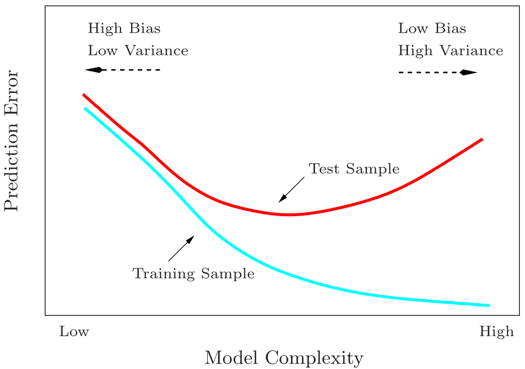
Figure 1: Test and training error as a function of model complexity
Jacknife Estimates
We will model our discussion on the work of Efron (1982). Note that:
- The \(\hat{θ}\) symbol is an estimate of the true quantity \(θ\)
- This is defined by the estimate being \(\hat{θ}=θ(\hat{F})\)
- \(\hat{F}\) is the empirical probability distribution, defined by mass \(1/n\) at \(xᵢ ∀ i∈I\), i is from 1 to n
The points above establishes our bias to be given by \(E_Fθ(\hat{F})-θ(F)\) such that \(E_F\) is the expectation under x₁⋯xₙ~F.
To derive the Jacknife estimate \((\tilde{θ})\) we will simply sequentially delete points xᵢ (changing \(\hat{F}\)), and recompute our estimate \(\hat{θ}\), which then simplifies to:
\begin{equation} \tilde{θ}\equiv n\hat{θ}-(\frac{n-1}{n})∑_{i=1}ⁿ\hat{θ} \end{equation}
In essence, the Jacknife estimate is obtained by making repeated estimates on increasingly smaller data-sets. This intuition lets us imagine a method which actually makes estimates on larger data-sets (which is the motivation for data augmentation) or, perhaps not so intuitively, on estimates on data-sets of the same size.
Bootstrap Estimates
Continuing with the same notation, we will note that the bootstrap is obtained by draw random data-sets with replacement from the training data, where each sample is the same size as the original; as noted by Hastie, Tibshirani, and Friedman (2009).
We will consider the bootstrap estimate for the standard deviation of the \(\hat{θ}\) operator, which is denoted by \(σ(F,n,\hat{\theta})=σ(F)\)
The bootstrap is simple the standard deviation at the approximate F, i.e., at \(F=\hat{F}\):
\begin{equation} \hat{\mathrm{SD}}=\sigma(\hat{F}) \end{equation}
Since we generally have no closed form analytical form for \(σ(F)\) we must use a Monte Carlo algorithm:
- Fit a non parametric maximum likelihood estimate (MLE) of F, i.e. \(\hat{F}\)
- Draw a sample from \(\hat{F}\) and calculate the estimate of \(\hat{θ}\) on that sample, say, \(\hat{θ}^*\)
- Repeat 2 to get multiple (say B) replications of \(\hat{θ}^*\)
Now we know that as \(B→∞\) then our estimate would match \(σ(\hat{F})\) perfectly, however, since that itself is an estimate of the value we are actually interested in, in practice there is no real point using a very high B value.
Note that in actual practice we simply use the given training data with repetition and do not actually use an MLE of the approximate true distribution to generate samples. This causes the bootstrap estimate to be unreasonably good, since there is always significant overlap between the training and test samples during the model fit. This is why cross validation demands non-overlapping data partitions.
Connecting Estimates
The somewhat surprising result can be proved when \(\hat{θ}=θ(\hat{F}\) is a quadratic functional, namely:
\begin{equation}\hat{\mathrm{Bias}}_{boot}=\frac{n-1}{n} \hat{\mathrm{Bias}}_{jack}\end{equation}
In practice however, we will simply recall that the Jacknife tends to overestimate, and the Bootstrap tends to underestimation.
Bagging
Bagging, is motivated by using the bootstrap methodology to improve the estimate or prediction directly, instead of using it as a method to asses the accuracy of an estimate. It is a representative of the so-called parallel ensemble methods where the base learners are generated in parallel. As such, the motivation is to reduce the error by exploiting the independence of base learners (true for mathematically exact bootstrap samples, but not really true in practice).
Mathematically the formulation of Hastie, Tibshirani, and Friedman (2009) establishes a connection between the Bayesian understanding of the bootstrap mean as a posterior average, however, here we will use a more heuristic approach.
We have noted above that the bagging process simply involves looking at different samples in differing orders. This has some stark repercussions for tree-based methods, since the trees are grown with a greedy approach.
- Bootstrap samples may cause different trees to be produced
- This causes a reduction in the variance, especially when not too many samples are considered
- Averaging, reduces variance while leaving bias unchanged
Practically, these separate trees being averaged allows for varying importance values of the variables to be calculated.
In particular, following Hastie, Tibshirani, and Friedman (2009), it is possible to see that the MSE tends to decrease by bagging.
\begin{align} E_P[Y-\hat{f}^*(x)]² & = & E_P[Y-f*{ag}(x)+f^*_{ag}(x)-\hat{f}^*(x)]² \\ & = & E_P[Y-f^*_{ag}(x)]²+E_P[\hat{f}^*(x)-f^*_{ag}(x)]² ≥ E_P[Y-f^*_{ag}(x)]² \end{align}
Where:
- The training observations are independently drawn from a distribution \(P\)
- \(f_{ag}(x)=E_P\hat{f}^*(x)\) is the ideal aggregate estimator
For the formulation above, we assume that \(f_{ag}\) is a true bagging estimate, which draws samples from the actual population. The upper bound is obtained from the variance of the \(\hat{f}^*(x)\) around the mean, \(f_{ag}\)
Practically, we should note the following:
- The regression trees are deep
- The greedy algorithm growing the trees cause them to be unstable (sensitive to changes in input data)
- Each tree has a high variance, and low bias
- Averaging these trees reduces the variance
Missing from the discussion above is how exactly the training and test sets are used in a bagging algorithm, as well as an estimate for the error for each base learner. This has been reported in the code above as the OOB error, or out of bag error. We have, as noted by Zhou (2012) and Breiman (1996) the following considerations.
- Given \(m\) training samples, the probability that the iᵗʰ sample is selected 0,1,2… times is approximately Poisson distributed with \(λ=1\)
- The probability of the iᵗʰ example will occur at least once is then \(1-(1/e)≈0.632\)
- This means for each base learner, there are around \(36.8\) % original training samples which have not been used in its training process
The goodness can thus be estimated using these OOB error, which is simply an estimate of the error of the base tree on the OOB samples.
As a final note, random forests are conceptually easily understood by combining bagging with subspace sampling, which is why in most cases and packages, we used bagging as a special case of random forests, i.e. when no subspace sampling is performed, random forests algorithms perform bagging.
References
Breiman, Leo. 1996. “Bagging Predictors.” Machine Learning 24 (2): 123–40. https://doi.org/10.1023/A:1018054314350.
Cichosz, Pawel. 2015. Data Mining Algorithms: Explained Using R. Chichester, West Sussex ; Malden, MA: John Wiley & Sons Inc.
Efron, Bradley. 1982. The Jackknife, the Bootstrap, and Other Resampling Plans. CBMS-NSF Regional Conference Series in Applied Mathematics 38. Philadelphia, Pa: Society for Industrial and Applied Mathematics.
Hastie, Trevor, Robert Tibshirani, and J. H. Friedman. 2009. The Elements of Statistical Learning: Data Mining, Inference, and Prediction. 2nd ed. Springer Series in Statistics. New York, NY: Springer.
James, Gareth, Daniela Witten, Trevor Hastie, and Robert Tibshirani. 2013. An Introduction to Statistical Learning. Vol. 103. Springer Texts in Statistics. New York, NY: Springer New York. https://doi.org/10.1007/978-1-4614-7138-7.
Zhou, Zhi-Hua. 2012. Ensemble Methods: Foundations and Algorithms. 0th ed. Chapman and Hall/CRC. https://doi.org/10.1201/b12207.
This is mostly true for reasonably smooth true functions ↩︎
![]()